Software2
Visualization
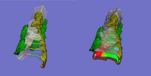
Data Analysis and Visualization Environment (DAVE) is our primary 3D visualization tool. DAVE help and some DAVE images are viewable online.
Simulation
analyze_simulation.pl -h
This program takes one or more outputs of a simulation (e.g. output of run1 or run2) For each z slice (time point) in each output: blurs it with a psf, pulls out the in-focus slice. Then calculates total concentration CHANGE (relative to time 0) as a function of distance from the calcium entry site (assumed to be the brightest point over all time after blurring). This is written to a file with the same root as the input simulation, but with a .xy extension. This can be viewed with xmgrace, or read into matlab (readxmgr) and visualized with acurves().
Assumes simulation was at 100 nm resolution. Uses a fixed psf with 300x300x150 nm voxels. Several scale factors are applied, so comparisons of magnitudes between files are not valid (but comparisons between time pts from the same file are fine).
analyze_simulation.pl [options] sim.i2i [additional input files]
options: -zrange=#:#:# startz stopz dz, inclusive, zero indexed. default is all z slices (i.e., all time pts). -verbose print out extra into to stderr as it goes along -keepfiles keep all intermediate files. may take lots of space!
examples: analyze_simulation.pl -verbose -zrange=0:10:1 run1_cafl.i2i > & sim.out
xmgrace run1_cafl.xy
matlab: data = readxmgr('run1_cafl.xy'); acurves(data);
analyze_simulation.pl -verbose run1_cafl.i2i run1_ca.i2i > & sim.out
calc_diffusion3.pl -h
   This program reads in a 2D diffusion tracks and calculates a D for each file (track_\d+.out)
   by fitting a line to the MeanSquaredDisplacement vs time:
MSD(t) = 4Dt (it would be MSD(t) = 4Dt + 2*sigma^2 if there is noise, see ref below).
   so the slope of the line divided by 4 should yield D (even in the case with noise).
   note: Lag intervals overlap one another unless -no_overlap is specified.
   meanD, varD, and standard error of the meanD is printed to stderr.
   note: if -no_overlap is not specified, the standard error of the mean (seD) may not be correct
         since the points aren't independent.
calc_diffusion3.pl [options]
-minlag=# if not specified, minlag = 1 -maxlag=# if not specified, maxlag = 1/2 the total time in the first track file analyzed -duration=# rather than analyze each track in its entirety, split it into (non-overlapping) sections of the specified duration (number of time points). -files=file1:...:filen list of filenames to analyze (instead of all track_#.out files)
-filerange=#:# only look at files track_#1.out to track_#2.out (inclusive)
-logfit also do the D calculation (via a line fit) in the log-log space (ln (MSD(t) = ln(4D) + ln(t)) -no_overlap
	-print_Ds	print all the Ds calculated, one per line (tracknum D), to stdout.
	-print_wDs	print all the weighted Ds calculated, one per line (tracknum D), to stdout.
-print_graph prints to stdout MSD vs time -notracknum the filename being read does not have tracknumber in it, just autonumber them. -dummy just print some info to stderr -verbose which file is being analyzed printed to stderr
   example:
       calc_diffusion3.pl  -print_graph files=track_1.xy | cull -c -s -1 -2 |xmgrs
# take a 1,000 pt track and analyze it as 10 separate 100 length tracks to see what those Ds look like:
       calc_diffusion3.pl  -print_Ds -print_wDs -files=track_1.xy
       calc_diffusion3.pl  -duration=100 -print_Ds -print_wDs -files=track_1.xy
see also:
calc_diffusion.pl same program but only operates on one file. calc_diffusion2.pl same program but without the -duration option SingleParticleTracking_DiffusionCoefficients_Saxton.pdf p. 1746 for the algorithm SubdiffusionOfSingleParticleTracks.pdf - p. 4 gives the formula if there is noise in the estimate.
compare_volume_measurements.pl -h
This program combines data produced by cross_sections_of_voronoi (-vfile) with an analysis of the same image within fiji (via the stereology_lml macro, -sfile). Results printed (on each line there will be sfile data then vfile data) to stdout.
compare_volume_measurements.pl [options] -vfile=filename1.txt -sfile=filename2.txt
options: -print_volumes rather than print entire combined lines, just print volume info in columns. the columns are: region: the region id, this is the same as the pixel value. sarea: the cross-sectional region area as reported by the fiji stereology_lml.txt macro. svolume: the volume estimated by stereology_lml.txt swvolume: the weighted volume estimated by stereology_lml.txt (not really a true volume). true_volume: the true volume of the region (as created by cross_sections_of_voronoi). area: area as reported by cross_sections_of_voronoi volume_from_area another way to estimate volume from area, w/out stereology: ((1/.68)*area)^(3/2) -vprefix=# foreach field printed out, change its name by adding the specified prefix -sprefix=# foreach field printed out, change its name by adding the specified prefix this may be used so that field names become unique (otherwise, eg, there will be two "area" fields and two "volume" fields on each line). -verbose stuff to stderr
examples: cross_sections_of_voronoi -P voronoi.i2i > filename1.txt Fiji Edit->options->conversions - make sure "scale when converting" is NOT checked.
            Plugins-> open i2i -> voronoi.i2i, then Image->type->32, Image->type->16, to get rid of the table lookup
            Plugins->macros->install... install stereology_lml.txt
            Plugins->macros->stereology_lml.txt  -> voronoi_fiji.txt
compare_volume_measurements.pl -vfile=filename1.txt -sfile=voronoi_fiji.txt
# look at volume estimated via stereology (x axis) vs. true volume (y axis): compare_volume_measurements.pl -print_volumes -vfile=filename1.txt -sfile=voronoi_fiji.txt | cull -c -s -3 -5 | xmgrace -free -pipe
# look at volume estimated from area (x axis) vs. true volume (y axis): compare_volume_measurements.pl -print_volumes -vfile=filename1.txt -sfile=voronoi_fiji.txt | cull -c -s -7 -5 | xmgrace -free -pipe
# compare true volume (x axis) to both the stereology estimated volume and the volume from area measurements (y axis): compare_volume_measurements.pl -print_volumes -vfile=filename1.txt -sfile=voronoi_fiji.txt | cull -c -s -5 -3 -7 > tmp.nxy
xmgrace -nxy tmp.nxy -free
see also: /home/lml/krypton/Corvera/Raz/stereology/README, run_voronoi.pl cross_sections_of_voronoi /home/lml/krypton/packages/fiji/Fiji.app/macros/stereology_lml.txt
filter_beads.pl -h
Reads in a file produced by makebeads2 (bead.info) and one produced by print_pixel_coords (mask.info). A bead's info is kept only if at least one of its voxels is under the mask. Kept beads are printed to stdout with their original values (bead id, position, etc.). Thus, if you actually mask the bead image (using maski2i) which was produced by makebeads2, this will keep the associated bead info for those beads which have at least one pixel left in the image after masking.
Note: this can only be run on data produced by versions of makebeads2 newer than 2/12/09.
filter_beads.pl bead.info mask.info > filtered_bead.info
options:
-keepcenter=# : rather than keep a bead if any of its voxels is under the mask, only keep the bead
if its center is under the mask. # is the scale factor to convert from the original resolution the bead was created at (-S option to makebeads2) and the resolution of the mask. For example: makebeads2 -S 0.005 0.005 0.005 ... > beads.info If you then use a mask at .1 um you would specify -keepcenter=20
-verbose
Example:
   makebeads2 -v -d 1280 1280 60 -S 0.005 0.005 0.005  -n 300 -i 1 beads300.i2i > bead.info
   maskimage beads300.i2i mask.i2i beads_masked.i2i
       # now want to filter bead.info to leave only beads at least partially under  mask.i2i (i.e., beads with at least one pixel
       # left in beads_masked.i2i)
   print_pixel_coords -2 mask.i2i > mask.info
   filter_beads.pl bead.info mask.info  > filtered_bead.info
# now filtered_bead.info "matches" what is left in beads_masked.i2i
An example where resolution is changed: # voxel coords printed to bead.info by makebeads2 will reflect the new (chres'ed) coords appropriately:
makebeads2 -v -d 1280 1280 60 -S 0.005 0.005 0.005 -c 0.025 0.025 0.01 -n 300 -i 1 beads.i2i > bead.info
# now actually change the res of the bead image to match:
chres -S 5 5 2 beads.i2i beads_ch.i2i
# apply the mask to the lower res image. mask must already be at that same resolution:
maskimage beads_ch.i2i mask_ch.i2i beads_ch_masked.i2i
# get out coords of all pixels in this low res mask:
print_pixel_coords -2 mask_ch.i2i > mask_ch.info
# now just keep the bead info for beads which are under the mask at this low resolution:
filter_beads.pl bead.info mask_ch.info > filtered_bead.info
# now filtered_bead.info "matches" what is left in beads_ch_masked.i2i (I hope!)
See also: makebeads2, print_pixel_coords
graph_xpp2.pl -h
Reads specified columns of data from an xpp output file. Sends output stdout.
note: time is always the first variable output (i.e., the first column).
usage:
graph_xpp2.pl [options] output.dat > name1_name2.dat
options:
-allstates: extract all columns of data having to do with channel state.
This is all the basic data. Other data is derived from this.
  -openstates:		all open states.  cannot be specified with -closedstates.
  -nopen:		sum of all the open states. cannot be used with -closedstates.
  -closedstates:	all closed states. cannot be specified with -openstates.
  -verbose
example:
  xpp -silent bk.ode    -> output.dat
  graph_xpp.pl -vars=time:name1:name5:name7 output.dat   > xpp_subset.out
  xmgrace -nxy xpp_subset.out
see also:
graph_xpp.pl
oxygen_krogh.pl -h
NOT DONE YET.
   Calculates steady state oxygen levels as a function of distance from a
   blood vessel (see ~/krypton/Corvera/Olga).
   Writes to (rstar,Pstar) columns to stdout; this is the Krogh-Erlang
   equation. Equation 17 of KroghOxygenDiffusionModel1.pdf
oxygen_krogh.pl [options]
options:
see also: oxygen_krogh.c
random_path.pl -h
Generate a random path (ie, diffusion).
usage:
random_path.pl [options] > track_1.out
options: -D=# diffusion coefficient, default = 1 -length=# pathlength (number of time points). default = 1000 -xy only print x,y rather than t,x,y
-method=oversample|gaussian oversample takes dt size substeps to calculate each 1 time unit step. gaussian just samples into an equivalent Gaussian distribution once for each 1 time unit step. default: oversample. gaussian option not tested yet... -dt=# substep time interval, default = .001 (only used if -method=oversample). -seed=# so random numbers are the same from run to run (only if -method=oversample)
note: using the default random number generator which is probably not great.
see also: run_random_path.pl calls random_path.pl to generate lots of paths. calc_diffusion3.pl can analyze these paths ~/krypton/diffusion/mytracks/
readbeads.pl -h
Reads in file produced by makebeads to check to see if sizes and amplitudes are Gaussian and Poission (-G and -P options). Produces _tmpsize and _tmpamp. You may want to use filterbeads.pl prior to using readbeads.pl. You can read these into xmgrace and then create histograms if so desired.
readbeads.pl makebeads.out
-skipzero skip values which are zero -outer put outer diameter (rather than "size") into _tmpsize. If makebeads used the -g option, then size always equals 1. outer should be the gaussian mean + 1/2 shell width. -rpts=# also prints out _coords.rpts file of coordinates of center of beads. This can be read in by addlines. Can also be read by pt_distances. # is a scale factor to divide by to get the new coordinates (so you can compare these to a lower resolution image). Set # to 1 if you don't want to scale the values. Note: coords are truncated an integer value (new = integer(old/# + 1)). skipzero command doesn't affect this option. note: if more than 1 point has the same new coordinates, then the w value for each duplicate point is 1 higher than the previous value (e..g, if -w=-10, then the first (5,6,3) has a w = -10, next has a value -9, next -8, etc. note: this also causes coords to be converted from 0-indexed (makebeads2 output) to 1-indexed (play assumes this for rpts files). -dontrescalez: when using -rpts=#, don't rescale the z coord -twod ignore z dimension when printing rpts file (still must specify -rpts option). -w=# in rpts file, set w to specified number, default = -1000 -amp use the amplitude of the bead for the w value in rpts file output
See also: filterbeads.pl, makebeads2, objs2dist121.pl, print_pixel_coords, filter_beads.pl
run_random_path.pl -h
Generate lots of random paths files (ie, diffusion) by calling random_path.pl multiple times..
usage:
run_random_path.pl [options]
options: -seed=# so random numbers are the same from run to run -D=# diffusion coefficient, default = 1 -length=# pathlength (number of time points). default = 1000 -xy only print x,y rather than t,x,y -numpaths=# default = 10 paths -rootname=string default: track_ (so files will be called track_#.out) -verbose stuff to stderr
note: using the default random number generator which is probably not great.
see also: random_path.pl calc_diffusion3.pl
run_voronoi2.pl -h
This script calls cross_sections_of_voronoi many times, and produces an image and output text file from each run.
run_voronoi2.pl [options]
options:
  -num=#	number of times to run. default = 10
  -D=#		-D option to cross_sections_of_voronoi, average diameter, default = 150
  -dummy	don't do anything, just echo to stderr what would be done
voronoi_vs_fiji.pl -h
compare the true volumes of voronoi regions (as reported by cross_sections_of_voronoi, e.g. voronoi_D170_0001_g0_G250_volume.txt) to those calculated within fiji using stereology_lml.txt (e.g., voronoi_D170_0001.txt)
Graphs volume (x) vs predicted volume (y) (or prints to stdout if -stdout is specified)
note: if looking at weighted volumes (eg, in weighted/ ), the individuals stereologic volumes
really are meaningless, and you should really just pull out the wmean values from each run.
usage:
voronoi_vs_fiji.pl [options] *volume.txt
options:
 	-vdir=/path/to/directory              location of directory with the output from cross_sections_of_voronoi
                                       (eg. voronoi_D170_0001.txt) default is the current directory
-debug info about all fields on each line printed to stderr
-stdout everything to stdout
-print_avg for each file, just graph mean and std error of the mean (gotten by combining all the data for each file, so may include multiple stereological runs) rather than all data pts note: this will average together the multiple fiji stereology runs which are often in the same *volume.txt file. I think that is ok (but may make the sem look better than it would be from just one run).
-use_wmean just use the mean or wmean stored in the *volume.txt file and compare these values to ??? ... not done yet
examples: cd /storage/big1/lml/Raz/voronoi run_voronoi2.pl -D=170 -num=20 # calls cross_sections_of_voronoi run_voronoi2.pl -D=220 -num=20 # calls cross_sections_of_voronoi Fiji # then run run_stereolgy_voronoi.ijm cd results/
       voronoi_vs_fiji.pl -vdir=..  *D170*volume.txt  # -> voronoi_vs_fij_D170.xmgr
       voronoi_vs_fiji.pl -vdir=.. *D220*volume.txt  # -> voronoi_vs_fij_D220.xmgr
see also:
/storage/big1/lml/Raz/voronoi/ - this is where I've done what is shown in the examples above
/storage/big1/lml/Raz/voronoi/README, true_vs_predicted.xmgr
/home/lml/krypton/Corvera/Raz/stereology/README, run_voronoi.pl, run_voronoi2.pl, compare_volume_measurements.pl, plot_results.pl
cross_sections_of_voronoi
/home/lml/krypton/packages/fiji/Fiji.app/macros/stereology_lml.txt
/home/lml/krypton/packages/fiji/run_stereology.txt
analyze_cross_sections_of_voronoi.pl
ball
incorrect command line. This program creates an elliptical shell of brightness the specified brightness (-i option) It is used to create test images for Fischer/hmc.
Usage: ball [options] ball.i2i options: -d xdim ydim zdim: dimensions of image, default = (50,100,50) -r x y z: x,y, and z radius in voxels, default = (20.000000,20.000000,20.000000) -s samplerate: number of subsamples in x and z directions per pixel, default = 1 -i intensity: intensity of the ball's shell, default = 100.000000 -b intensity: intensity background voxels, default = 0.000000 -f image: read in the specified image, add the ball image to that (just replaces voxels along the ball's shell with new values). -t thickness: thickness of shell, default = 1.000000
Note: you can call this multiple times to get a shell within a shell
code in /home/lml/krypton/facil/ball.c
calc_ca3
- /home/lml/krypton/bin/calc_ca3
incorrect command line. Reads in 4 floating point images (or 4 short int images) as produced by simulation, calculates the difference image deltaca.i2i (as a floating pt image) between the observed free calcium and what would be expected in equilibrium conditions, i.e., [ca]-[predicted_ca], where [predicted_ca]
is kd*[CaFl]/[Fl]. Output concentration in nM.
All input concentrations should be in nM Each z slice is analyzed separately (i.e., z is assumed to be time).
Usage: calc_ca3 [options] ca.i2i fl.i2i cafl.i2i cafixed.i2i deltaca.i2i options: -k #: kd in uM, default = 1.125000
        -h:		print cumulative histogram for each z slice.
      options for printing graphs of free calcium (not concentration) vs. distance from ca entry location:
the units for the graph are nM*um^3, but 1nM = .6ions/um^3 , so multiply be .6 to get ions
                      (and 1pA = 3,000 ions/msec if you want to convert to pA-msec).
        -c:		print delta calcium (delta from first slice) distance graph for each z slice.
        -n:		normalize delta calcium distance graph for each z slice (so sum of amplitudes = 1),
                      (otherwise when graph spacing is changed, -g option, the height of the graph will change).
        -a:		print absolute calcium, not delta calcium.
                      when this is applied to a uniform image it should produce a 4pi*r*r distribution.
      options for printing graphs of total calcium, i.e. ca+cafl+cafixed (not concentration):
        -C:		print delta total calcium distance graph for each z slice.
        -N:		normalize delta total calcium distance graph for each z slice (so sum of amplitudes = 1).
        -A:		print absolute total calcium, not delta total calcium
-p # #: pixel size in microns in the radial (x) and lengthwise (y) directions, default = 0.10 and 0.10 -P # # #: pixel size in microns in x,y,z directions (rectangular not cylindrical coords), default = ( 0.10, 0.10, 0.10) -r: data is rectangular, not cylindrical coords (-P sets this too) -e x y: 0-indexed coords of calcium entry location (default: x= 0, y = ydim/2)
        -g #:		graph spacing for -c,-C,-n,-N,-a,-A options. defauls is pixel size.
        -s #:         subsample each voxel this number of times in the x (radial) and y (longitudinal) directions,
                      default = 3.  Subsampling only applies to histogram and graph generation, not image generation.
        -z low hi dz: only look at z slices low to hi (0-indexed, inclusive), stepping by dz.
                      The zdim of deltaca.i2i will not change, but skipped slices will be 0.
see also:
float2int, in matlab: readxmgr, acurves (see ~lml/krypton/JSinger for an example)
source code in ~lml/krypton/Walsh directory.
cellsim -h
[0]: in main, before MPI_Init()
[0]: in main, after MPI_Init() [0]: /home/lml/krypton/bin/cellsim -h help: unable to parse command: -h
   This program simulates Ca and Na in a cylindrical cell with
   cylindrical symmetry.
   Note: It is recommended that the stderr output be examined for
         lines with the words: warning, Warning, error, or Error on them.
Usage
cellsim [options] >& output_datafile
Options controlling the duration of the simulation:
    -time #:       total time to simulate (in sec), default = 0.000000
    -time_rate #:  slow down time, ie take smaller dt steps during simulation.
                   this may be necessary if you are creating a large ca gradient,
                   for example, with -ca_ring or -ca_src options (.5 means 1/2 the dt).
                   The number of iterations needed for convergence is
                   roughly: I= (T*diff)/(dr*dr), where T is time, dr is
                   annulus thickness and diff is diffusion constant.
                   This ignores ion influx,etc.  If you set diffusion rates very
                   small, the iter # calculated will be too small if other stuff
                   is happening, use -time_rate to compensate.
Options controlling the geometry of the model:
    -radius #:     radius of the cell in microns, default = 6.000000
    -rings #:      radius of the cell in rings, default = 60
                   Ring thickness = cell radius/ # of rings.
    -length #:     length of the cell in disks, default = 300
                   Each disk will be the same thickness as a ring.
    -bc Rmax Lmin Lmax:     boundary conditions at maximum radius and minimum and
                   maximum length coordinate (i.e., at the cell ends). These must
                   be the letters I (for infinite) or S (for solid, i.e. no ions go
                   through the membrane). The I option is not always accurate. default: S
    -mask image.i2i: only voxels in image.i2i > 0 are part of the cell.  Use this
                   to specify an arbitrary shape for the cell.
                   Not extensively tested.
    -spacing file: file specifies the spacing along each axis (i.e, size of each voxel).
                   spacing is in nm, one entry per voxel, comment lines ignored (#).
                   The cell direction (X,Y, or Z) must be the first letter on the line.
                   Other characters on the line will be ignored.
                   The number of entries must be < 2000 each direction.
                   Do not specify -rings,-radius,and -length if you use this option.
                   NOTE: the simulation time step goes as (length)^2, where length is
                         the length of the shortest side of all the voxels specified.
                   Any number of entries per line. First R, then D (length). Example:
                   # R direction (10 pixels in this direction, high res at low R)
                   X
                   25 50 75 100 200 300 400 500 600 1000
                   Y (lengthwise) direction (9 pixels in D, very high res in the middle)
                   100 200 300 400 500 540 550 560 1000
                   Use cyl2cart with -spacing option to convert output images to
                   a uniform spacing. (I haven't added that option yet)
                   Not extensively tested.
Options specifying substances (ions, buffers, compounds) present in the model (10 max):
    -ion name free_concentration D valence:
                   concentration in mMolar, D in cm^2/sec, valence in absolute value.
                   valence is only used if -ion_src is also specified.
                   concentration is the initial free concentration.
    -buffer name total_concentration D:
                   concentration in mMolar, D in cm^2/sec.
                   concentration is the initial total concentration (sum of its free and all bound forms).
    -kin bufname ionname boundname onrate offrate D:
                   kinetics for interaction between bufname and ionname.  Boundname is the
                   name to give the bound pair.  bufname and ionname must have been
                   specified (with -ion -buffer or -kin options) prior to this option.
                   onrate:in 1/(mMolar*seconds), offrate: in 1/seconds, D: in cm^2/sec
    -equil_error relerr iter: maximum relative equilibrium error allowed during the
                   initial calculation of concentrations from the user specified
                   free ion concentrations and total buffer concentrations.
                   rel_error = ABS((true_kd - calculated_kd)/true_kd). Default = 1e-05
                   This should be small enough unless you have huge buffer
                   concentrations (>100 mM?). iter (an int) is maximum number of iterations
                   to allow during equilibration, max =1 billion, default = 10000000
Options controlling changing conditions:
    -ion_src name current dur lowdisk highdisk lowring highring:
                   have a current source of the specified ion coming in through the specified rings
                   and numdisk (rings and disks are 0-indexed indices, inclusive).
                   Current is in pA for the specified duration (sec).
                   The current is uniformly divided within the entire specified input volume.
                   All -buffer and -ion options must be specified prior to this.
                   See comments by the -time_rate option.
    -ion_src_file name imagename current duration:
                   Similar to -ion_src, but the specified floating point image is used to
                   scale the input current at each voxel. The total current coming into the
                   cell is adjusted so that after this per pixel rescaling, it will = "current".
                   -ion_current_trace with op = S, will modify this.
                   Typically do: int2float -M 1 psf.i2i imagename        prior to this.
    -ion_current_trace name filename dt op threshold:  modifies current specified with
                   the -ion_src or -ion_src_file options.
                   Times which the channel is open (i.e., current flows) is specified in a file.
                   The file is a list of numbers (current or scale), 1 per line, at dt (in sec) intervals.
                   If op = T, currents greater than the specified threshold means channel open, otherwise closed.
                   If op = S, the current as specified with -ion_src is scaled by the number in the list.
                   "threshold" is required but ignored when op = S.  Not extensively tested.
    -zap_sub name time:
                   At the specified time (in seconds) set the named substance concentration
                   to 0. This does not prevent it from being produced from other reactions.
                   This is useful if an injected "ion" was photons (e.g., photon+caged -> uncaged)
                   and the laser is turned off at the specified time.
    -ion_pump name max_rate n k lowdisk highdisk lowring highring:
                   have a pump of the specified ion remove ions in the specified rings
                   and numdisks (rings and disks are 0-indexed indices, inclusive).
                   max_rate * [ion]^n / (k^n + [ion]^n),  [ion] and k in mM. max_rate in mM/sec.
max rates are typically given per unit area (8E-7 umoles/(cm^2 sec) for serca pump). If we divide these published numbers by the ring width (typically 100 nm) we can get a rough rate per unit volume. A typical max_rate might be .1 mM/sec (seems high, Polito et al. biophysj, May, 2006 give a rate in terms of []/volume of ~ .001 mM/sec - but they also have a k on the low end, .0001mM, which would compensate some. Shuai & Jung, PNAS, Jan. 21,2003, p. 507 have a max rate of .5 (uM?)/sec.) Typical values for k might be around .0001-.0005 mM. n=2 for serca pump (must be integer)
                   All -buffer and -ion options must be specified prior to this.
    -ion_leak name rate compartment_conc lowdisk highdisk lowring highring:
                   have a leak of the specified ion introduce ions into the specified rings
                   and numdisks (rings and disks are 0-indexed indices, inclusive).
                   rate * ([compartment_conc] - [ion]),  [] in mM. rate in 1/sec.
Leak rates are usually set to exactly balance the pump at initial ion concentrations. compartment_conc for [ca] in the SR might be around 2 mM. If max_rate = .001mM/sec, k = .0005mM, compart_conc = 2mM, and resting [ca] = 100nM, rate should = .00001923/sec to balance the pump with the leak. note: Leaks INTO the compartment (when [ion]_in_cyto>compartment_conc) are not allowed.
All -buffer and -ion options must be specified prior to this.
Options related to output:
    -save name filename type scale dt:
                   Save images of the specified substance (name) to specified file. By default
                   substances are saved in mM.  This will be multiplied by the scale
                   specified here. dt (in sec) is how often to save images.  Type is I
                   (short int, our normal format) or F (floating pt,2x space, more accurate).
                   The first image saved will be prior to any ion current. The last image
                   will always be the end of the simulation. "name" should be as
                   specified with the -ion, -buffer or -kin option.
                   If the image file already exists, new images will postpended to it.
    -save all tag type scale dt:
                   Equivalent to -save for all ions and buffers. Uses default file names,
                   but adds the tag on the end. ions in nM, all else in uM, then times scale.
    -save_flow name rfilename lfilename scale dt:
                   Save flow images of the specified substance (name) to specified files.
                   rfile is radial flow, lfile is lengthwise flow. Images saved in floating pt.
                   Flow is in pA (1 pA = 3 molecules/usec) times scale.
                   dt (in sec) is how often to save images.
    -save_flow all ltag rtag scale dt:
                   Equivalent to -save_flow for all ions and buffers. Uses default file names,
                   but adds the tag on the end. Output same scale as above.
                   NOTE: flow for EACH substance takes 8*(number of voxels) of space.
    -debug #:      set debug level to #. May substantially slow down the simulation.
                   1: extra print statements at init. 2: more testing while running. 3:
    -debug_subvolume #: Normally the total mmoles (in the entire cell) of each saved substance is
                   printed to stderr.  Setting this option will also cause the printing of the
                   total over a subvolume. Subvolume is all y >= # (0-indexed).
                   Example: if a cell has patch region at y=[1,10], setting # to the neck (11) of the
                   patch will let you see how much actually gets out into the main part of the cell.
Options related to MPI (multiprocessor stuff):
    invoke on the wolves as, for example,  mpirun -np 3 -machinefile file_of_machine_names cellsim ...
    -print_proc #:   only print output from the specified process (0 indexed).
                  Some output (eg, Total mmoles of ions, etc) are only valid for process 0.
    -overlap #:   overlap neighboring regions by the specified number of voxels (default = 50)
                  This will also be the number of iterations between necessary synchronization.
    -debug_mpi #:  print MPI info. Execute MPI dummy stubs if MPI NOT present (eg, under Windows,SGI).
                  This version of the executable does NOT use MPI.
    -debug_mpi_proc rank numproc:  set dummy rank and number of processes. use only if MPI NOT present!
EXAMPLES ./cellsim -time .0010 -time_rate .5 -length 200 -rings 40 -radius 1 \
       -ion Ca 100E-6 2.5E-6 2 -buffer Fluo3 .050 2.5E-7 -buffer Buf .230 1E-14  \
       -kin Fluo3 Ca CaFl 8E4 90 2.5E-7 -kin Buf Ca CaBuf 1E5 100 1E-14        \
       -ion_src Ca 1 .00105 99 102 0 3 \
       -save all _run1 I 1 .0001 >& cellsim_run1.out
Simulate for 100msec saving images every msec. 1 pA comes in the the pattern as specified
by psf_float.i2i for 10 msec. The current is then modulated by values in current.txt which
are one value per line, dt of 1 msec between them. Cell shape in mask.i2i. Voxel sizes in
spacing.txt
./cellsim -time .100 -time_rate .5 -spacing spacing.txt -mask mask.i2i \
       -ion Ca 100E-6 2.5E-6 2 -buffer Fluo3 .050 2.5E-7 -buffer Buf .230 1E-14  \
       -kin Fluo3 Ca CaFl 8E4 90 2.5E-7 -kin Buf Ca CaBuf 1E5 100 1E-14        \
       -ion_src_file Ca psf_float.i2i 1 .010 \
       -ion_current_trace Ca current.txt .001 S 999 \
       -save CaFl cafl.i2i I 1000 .001 -save Ca ca.i2i I 1E6 .001 \
       -save_flow Ca ca_radial_float.i2i ca_long_float.i2i 1 .001 >& cellsim.out
SEE ALSO
      ~lml/vision/bin/float2int                    (convert a floating point image to standard SHORT INT format)
      ~lml/vision/bin/int2float		      (convert normal image to floating point)
      ~lml/vision/bin/playexact                    (to display a floating point image)
      ~lml/invitro/Kargacin/changeheader           (change header of floating point image)
      ~lml/vision/bin/cyl2cart                     (convert from cylindrical to cartesian coords)
      ~lml/vision/bin/nadiffl7                     (many more options, but only 1 ion and 2 buffers)
      ~lml/vision/bin/diffuse2                     (simple Gaussian spot diffusion program)
      ~lml/invitro/Kargacin/iplot                  (3D graph of a 2D image, intensity -> height)
      ~lml/invitro/Kargacin/blur4D_dFoverF         (blur with psf, calculate dFoverF)
      ~lml/invitro/Kargacin/diffusion_limited_binding  (simulate diffusion limited binding)
      ~lml/invitro/Kargacin/spot_diffusion         (simulate diffusion from a spot)
      ~lml/vision/facil/printvals                  (print image values, calculate dFoverF)
      ~lml/vision/JSinger/src/channel              (steady state based upon Neher paper)
cellsimL -h
[0]: in main, before MPI_Init()
[0]: in main, after MPI_Init() [0]: /home/lml/krypton/bin/cellsimL -h help: unable to parse command: -h
   This program simulates Ca and Na in a cylindrical cell with
   cylindrical symmetry.
   Note: It is recommended that the stderr output be examined for
         lines with the words: warning, Warning, error, or Error on them.
Usage
cellsim [options] >& output_datafile
Options controlling the duration of the simulation:
    -time #:       total time to simulate (in sec), default = 0.000000
    -time_rate #:  slow down time, ie take smaller dt steps during simulation.
                   this may be necessary if you are creating a large ca gradient,
                   for example, with -ca_ring or -ca_src options (.5 means 1/2 the dt).
                   The number of iterations needed for convergence is
                   roughly: I= (T*diff)/(dr*dr), where T is time, dr is
                   annulus thickness and diff is diffusion constant.
                   This ignores ion influx,etc.  If you set diffusion rates very
                   small, the iter # calculated will be too small if other stuff
                   is happening, use -time_rate to compensate.
Options controlling the geometry of the model:
    -radius #:     radius of the cell in microns, default = 6.000000
    -rings #:      radius of the cell in rings, default = 60
                   Ring thickness = cell radius/ # of rings.
    -length #:     length of the cell in disks, default = 300
                   Each disk will be the same thickness as a ring.
    -bc Rmax Lmin Lmax:     boundary conditions at maximum radius and minimum and
                   maximum length coordinate (i.e., at the cell ends). These must
                   be the letters I (for infinite) or S (for solid, i.e. no ions go
                   through the membrane). The I option is not always accurate. default: S
    -mask image.i2i: only voxels in image.i2i > 0 are part of the cell.  Use this
                   to specify an arbitrary shape for the cell.
                   Not extensively tested.
    -spacing file: file specifies the spacing along each axis (i.e, size of each voxel).
                   spacing is in nm, one entry per voxel, comment lines ignored (#).
                   The cell direction (X,Y, or Z) must be the first letter on the line.
                   Other characters on the line will be ignored.
                   The number of entries must be < 2000 each direction.
                   Do not specify -rings,-radius,and -length if you use this option.
                   NOTE: the simulation time step goes as (length)^2, where length is
                         the length of the shortest side of all the voxels specified.
                   Any number of entries per line. First R, then D (length). Example:
                   # R direction (10 pixels in this direction, high res at low R)
                   X
                   25 50 75 100 200 300 400 500 600 1000
                   Y (lengthwise) direction (9 pixels in D, very high res in the middle)
                   100 200 300 400 500 540 550 560 1000
                   Use cyl2cart with -spacing option to convert output images to
                   a uniform spacing. (I haven't added that option yet)
                   Not extensively tested.
Options specifying substances (ions, buffers, compounds) present in the model (10 max):
    -ion name free_concentration D valence:
                   concentration in mMolar, D in cm^2/sec, valence in absolute value.
                   valence is only used if -ion_src is also specified.
                   concentration is the initial free concentration.
    -buffer name total_concentration D:
                   concentration in mMolar, D in cm^2/sec.
                   concentration is the initial total concentration (sum of its free and all bound forms).
    -kin bufname ionname boundname onrate offrate D:
                   kinetics for interaction between bufname and ionname.  Boundname is the
                   name to give the bound pair.  bufname and ionname must have been
                   specified (with -ion -buffer or -kin options) prior to this option.
                   onrate:in 1/(mMolar*seconds), offrate: in 1/seconds, D: in cm^2/sec
    -equil_error relerr iter: maximum relative equilibrium error allowed during the
                   initial calculation of concentrations from the user specified
                   free ion concentrations and total buffer concentrations.
                   rel_error = ABS((true_kd - calculated_kd)/true_kd). Default = 1e-05
                   This should be small enough unless you have huge buffer
                   concentrations (>100 mM?). iter (an int) is maximum number of iterations
                   to allow during equilibration, max =1 billion, default = 10000000
Options controlling changing conditions:
    -ion_src name current dur lowdisk highdisk lowring highring:
                   have a current source of the specified ion coming in through the specified rings
                   and numdisk (rings and disks are 0-indexed indices, inclusive).
                   Current is in pA for the specified duration (sec).
                   The current is uniformly divided within the entire specified input volume.
                   All -buffer and -ion options must be specified prior to this.
                   See comments by the -time_rate option.
    -ion_src_file name imagename current duration:
                   Similar to -ion_src, but the specified floating point image is used to
                   scale the input current at each voxel. The total current coming into the
                   cell is adjusted so that after this per pixel rescaling, it will = "current".
                   -ion_current_trace with op = S, will modify this.
                   Typically do: int2float -M 1 psf.i2i imagename        prior to this.
    -ion_current_trace name filename dt op threshold:  modifies current specified with
                   the -ion_src or -ion_src_file options.
                   Times which the channel is open (i.e., current flows) is specified in a file.
                   The file is a list of numbers (current or scale), 1 per line, at dt (in sec) intervals.
                   If op = T, currents greater than the specified threshold means channel open, otherwise closed.
                   If op = S, the current as specified with -ion_src is scaled by the number in the list.
                   "threshold" is required but ignored when op = S.  Not extensively tested.
    -zap_sub name time:
                   At the specified time (in seconds) set the named substance concentration
                   to 0. This does not prevent it from being produced from other reactions.
                   This is useful if an injected "ion" was photons (e.g., photon+caged -> uncaged)
                   and the laser is turned off at the specified time.
Options related to output:
    -save name filename type scale dt:
                   Save images of the specified substance (name) to specified file. By default
                   substances are saved in mM.  This will be multiplied by the scale
                   specified here. dt (in sec) is how often to save images.  Type is I
                   (short int, our normal format) or F (floating pt,2x space, more accurate).
                   The first image saved will be prior to any ion current. The last image
                   will always be the end of the simulation. "name" should be as
                   specified with the -ion, -buffer or -kin option.
                   If the image file already exists, new images will postpended to it.
    -save all tag type scale dt:
                   Equivalent to -save for all ions and buffers. Uses default file names,
                   but adds the tag on the end. ions in nM, all else in uM, then times scale.
    -save_flow name rfilename lfilename scale dt:
                   Save flow images of the specified substance (name) to specified files.
                   rfile is radial flow, lfile is lengthwise flow. Images saved in floating pt.
                   Flow is in pA (1 pA = 3 molecules/usec) times scale.
                   dt (in sec) is how often to save images.
    -save_flow all ltag rtag scale dt:
                   Equivalent to -save_flow for all ions and buffers. Uses default file names,
                   but adds the tag on the end. Output same scale as above.
                   NOTE: flow for EACH substance takes 8*(number of voxels) of space.
    -debug #:      set debug level to #. May substantially slow down the simulation.
                   1: extra print statements at init. 2: more testing while running. 3:
    -debug_subvolume #: Normally the total mmoles (in the entire cell) of each saved substance is
                   printed to stderr.  Setting this option will also cause the printing of the
                   total over a subvolume. Subvolume is all y >= # (0-indexed).
                   Example: if a cell has patch region at y=[1,10], setting # to the neck (11) of the
                   patch will let you see how much actually gets out into the main part of the cell.
Options related to MPI (multiprocessor stuff):
    invoke on the wolves as, for example,  mpirun -np 3 -machinefile file_of_machine_names cellsim ...
    -print_proc #:   only print output from the specified process (0 indexed).
                  Some output (eg, Total mmoles of ions, etc) are only valid for process 0.
    -overlap #:   overlap neighboring regions by the specified number of voxels (default = 50)
                  This will also be the number of iterations between necessary synchronization.
    -debug_mpi #:  print MPI info. Execute MPI dummy stubs if MPI NOT present (eg, under Windows,SGI).
                  This version of the executable does NOT use MPI.
    -debug_mpi_proc rank numproc:  set dummy rank and number of processes. use only if MPI NOT present!
EXAMPLES ./cellsim -time .0010 -time_rate .5 -length 200 -rings 40 -radius 1 \
       -ion Ca 100E-6 2.5E-6 2 -buffer Fluo3 .050 2.5E-7 -buffer Buf .230 1E-14  \
       -kin Fluo3 Ca CaFl 8E4 90 2.5E-7 -kin Buf Ca CaBuf 1E5 100 1E-14        \
       -ion_src Ca 1 .00105 99 102 0 3 \
       -save all _run1 I 1 .0001 >& cellsim_run1.out
Simulate for 100msec saving images every msec. 1 pA comes in the the pattern as specified
by psf_float.i2i for 10 msec. The current is then modulated by values in current.txt which
are one value per line, dt of 1 msec between them. Cell shape in mask.i2i. Voxel sizes in
spacing.txt
./cellsim -time .100 -time_rate .5 -spacing spacing.txt -mask mask.i2i \
       -ion Ca 100E-6 2.5E-6 2 -buffer Fluo3 .050 2.5E-7 -buffer Buf .230 1E-14  \
       -kin Fluo3 Ca CaFl 8E4 90 2.5E-7 -kin Buf Ca CaBuf 1E5 100 1E-14        \
       -ion_src_file Ca psf_float.i2i 1 .010 \
       -ion_current_trace Ca current.txt .001 S 999 \
       -save CaFl cafl.i2i I 1000 .001 -save Ca ca.i2i I 1E6 .001 \
       -save_flow Ca ca_radial_float.i2i ca_long_float.i2i 1 .001 >& cellsim.out
SEE ALSO
      ~lml/vision/bin/float2int                    (convert a floating point image to standard SHORT INT format)
      ~lml/vision/bin/int2float		      (convert normal image to floating point)
      ~lml/vision/bin/playexact                    (to display a floating point image)
      ~lml/invitro/Kargacin/changeheader           (change header of floating point image)
      ~lml/vision/bin/cyl2cart                     (convert from cylindrical to cartesian coords)
      ~lml/vision/bin/nadiffl7                     (many more options, but only 1 ion and 2 buffers)
      ~lml/vision/bin/diffuse2                     (simple Gaussian spot diffusion program)
      ~lml/invitro/Kargacin/iplot                  (3D graph of a 2D image, intensity -> height)
      ~lml/invitro/Kargacin/blur4D_dFoverF         (blur with psf, calculate dFoverF)
      ~lml/invitro/Kargacin/diffusion_limited_binding  (simulate diffusion limited binding)
      ~lml/invitro/Kargacin/spot_diffusion         (simulate diffusion from a spot)
      ~lml/vision/facil/printvals                  (print image values, calculate dFoverF)
      ~lml/vision/JSinger/src/channel              (steady state based upon Neher paper)
channel_current2
channel_current2: like channel_current, but looks at [ca] over time at each BK (not just max [ca]). From that, it calculates the max BK current. Channel_current adds the max [ca] that each BK voxel sees from each voxel in a Ryr cluster, to get the max [ca] that BK pixel sees. But the max [ca] could occur at different times since the Ryr cluster has a spatial extent. Experimental.
Calculates the current which would be produced when each object in Ryr_image.i2i releases calcium which activates nearby BK channels in BK_image.i2i. Produces a histogram of these output currents. The input images should have each pixel in an object having the object id as its value. These images can be produced with "countobjs -Q" or "objs_via_ascent" note: a one pixel border around the image is ignored (added 12/8/09). This may take about one-half hour to run.
Usage: channel_current [options] -f filename Ryr_image.i2i BK_image.i2i > im1_im2.hist Options: -f filename resting: file containing [ca], in nM, as a function of distance and time. Right now this is assumed to have 20 nm spacing and entries every msec. See /home/lml/krypton/Zhuge/STIC/simulations/run32.ca as an example "resting" is the resting [ca], in nM, for the cell. It will we subtracted from the other [ca] values to produce a "delta" [ca] which gets scaled linearly by Ryr intensity. The spark current used to produce this (see -C) should be roughly in the range expected for Ryr_image.i2i, since all delta [ca] is linearly extrapolated. All distances > largest distance in filename will have their [ca] set to the [ca] at the largest distance in filename. note: Only the [ca] values at y == 1 are used. Is this what should be used? -u #: voltage (mV). BK conductance is a function of voltage. default = -80.000000 -U low delta hi: voltages from low to hi by delta. Max is 20 voltages -r #: resolution (binsize) for output histogram in femtoAmps, default = 1000.000000 -R #: reveral potential of BK channel in mV, default = -80.000000
distances:
-w # # #: x,y, zweights for pixel distances (ie, pixel size), default = 1 for each. -p #: pixel size in nm (i.e., what 1 means in -w option), default = 80.000000 -m # : maxdistance (in units used for -w, i.e., pixels) to look for the closest pixel, default = 10.000000
which pixels or clusters to include:
-t # #: image1 and image2 thresholds, pixels > # are above threshold, default = 0. -e lowx lowy lowz hix hiy hiz: only look at voxels within this extent (subvolume), 1-indexed, inclusive. -s minsize maxsize: only look at objects in Ryr_image.i2i within the size range (inclusive, in voxels) max size allowed = 100000 -S minsize maxsize: only look at objects in BK_image.i2i within the size range (inclusive, in voxels) -i miniod maxiod: only look at objects in Ryr_image.i2i within the iod range (inclusive. use -d also.) -I miniod maxiod: only look at objects in BK_image.i2i within the iod range (inclusive. use -D also.)
scale factors:
-d Ryrimage1d.i2i #: the original intensity image for Ryr_image (since Ryr_image has pixel values as id numbers) # is the number of Ryrimage1d.i2i intensity units required to produce spark current used in the calcium simulation (which produced the -f filename data). This will scale the [ca] produced by each Ryr voxel. Default = 30000.000000 -D BKimage2d.i2i #: the original intensity image for BK_image (since BK_image has pixel values as id numbers) # is the BKimage2d.i2i intensity from one BK channel. This will scale current produced. Default = 1000.000000 If you want the intensity of each Ryr or BK object to affect the ca release (for Ryr) or number of channels (for BK) , you need to provide the original data by using the -d and -D options. Otherwise all voxels in an object contribute equally (so large objects have more receptors or channels than small ones). -c #: BK single channel conductance in pS, default = 220.0 -C #: peak current (in pAmps) used in the simulation to produce -f filename, default = 1.000000 This is just used for output produced by -v to estimate spark current produced per Ryr cluster.
  miscellaneous:
 	-v: 			verbose. produces list of each Ryr cluster and K current produced to stderr. Other stuff too.
To write this to a separate file do: (channel_current -v ... > stdout.channel) >& stderr.channel
-V: very verbose
Examples:
cellsim -spacing /home/lml/krypton/Zhuge/STIC/simulations/spacing2.txt .... : produces ca.i2i printvalsL -spacing2.txt -R -t -i ca.i2i > ca.vals kate ca.vals : delete fist comment line
objs_via_ascent -s 5 100 Ryr.i2i Ryrid.i2i > tmp
tail tmp : the mean IOD gives an idea of brightness needed to produce current used in cellsim, say 30000
objs_via_ascent -s 5 100 BK.i2i BKid.i2i > tmp
tail tmp : the mean IOD gives an idea of brightness of a BK cluster, eg mean= 10000, but assume that's 10 channels
channel_current -f ca.vals -w 1 1 3 -d Ryr.i2i 30000 -D BK.i2i 1000 Ryrid.i2i Bkid.i2i > ryr_bk.info cull -s -c -1 -4 < ryr_bk.info |xmgrace -source stdin See also: closest_object closest_voxel objs_via_ascent /home/lml/krypton/Zhuge/BKandRyr/graph.pl,match.pl graph_channel_current.pl, test_channel_current, /home/lml/krypton/Zhuge/STIC/simulations/run32 /home/lml/krypton/Zhuge/BKandRyr/analysis6/cluster_distances.pl, plot_mean_sd_curve.pl /home/lml/krypton/Zhuge/xpp/ASM15.ode Bugs:
Source code in ~krypton/lml/facil
# Popen is monotonic as it should be.
must provide -f cafilename
cluster -h
Drops random Ryr receptors into a world. Then calculates how many clusters and their sizes get produced. Currently the "world" default size is (2um)^3. (see -wsize) The origin of this world is in it's center (so it goes from -1um to +1 um in each direction by default). A histogram of cluster sizes is printed to stdout.
Usage: cluster [options] Options: distance options: -eucliddist: calculate a Euclidean distance (same in x,y,z directions). This is the default. (use -cdist option to set the nearby distance for this). -absdist: rather than calculate a real distance, calculate max(ABS(dx),ABS(dy),ABS(dz)) - for speed (use -cdist to set the nearby distance for this.) -psfdist x y z: distance (in um) a pt can be in the x, y, and z directions and be considered nearby. Does not use -cdist. To approximate a psf you might specify .2 .2 .6
-cdist #: how close (in um) two receptors must be to cluster, default = 0.500000
other options:
-2D: do a 2D simulation (x and y), not a 3D simulation
-cylinder inner outer: only place Ryr within a cylinder (e.g., plasma membrane) with specified
inner and outer radius (in um). The cylinder has its length the entire y dimension.
Only the parts of the cylinder which fit in the world (-wsize) are used. -wsize x y z: the width of the world (in um) in the x, y, and z directions (default = 2.0,2.0,2.0) -psize x y z: pixel width (in um) in the x, y, and z directions (default = 0.1,0.1,0.1)
-numryr #: number of Ryr receptors to drop, default = 1000
-mindist #: when placing Ryr receptors, keep this minimum distance (in um) between them. -randstart #: start the random number generator with # as the seed. So runs can be reproduced. -image name.i2i write out an image of the Ryr receptors. Can then use blur3d to create a realistic microscope image, and countobjs to analyze it and compare to real data. diagnostics:
      -debug:           turn on debugging
      -verbose:         be a bit more verbose
      -h:   print this help
      -H:   print this help
      -help:   print this help
Examples:
Source code in ~krypton/lml/Zhuge/Ryr_clusters
/home/lml/krypton/bin/cluster -h
diffusion_limited_binding -h
unknown option h incorrect command line. Prints out distance (um) and concentration (particles/cm^3) at that distance a slab volume of initial uniform concentration (1 particle/cm^3)which has a ligand binding to a plane at x = 0. This is diffusion limited binding. See my notes of 10/20/98.
Usage: diffusion_limited_binding [options] options: -D #: diffusion (cm^2/msec), default = 2.2E-09 -t t1 t2: start and stop time to simulate (msec), default = 0.000000 1000.000000 set both numbers equal if you only want one time point. -x x1 x2: start and stop distances to print (um), default = 0.000000 10.000000 set both number equal if you only want one position -L #: thickness of slab volume (um), default = 10.000000 -T #: number of samples in t, default = 10 -X #: number of samples in x, default = 1000 -h: print this help message. -F: print out time (msec) and flux (particles/cm^2-msec) at x = 0 (i.e., rate molecules binding to x=0 surface). I've made flux towards lower x positive (normally it would be negative). -B: print out time (msec) and total # of particles/cm^2 bound at x = 0 (i.e., brightness of surface). Integral of flux from t1 = 0 regardless of -t option setting. -s: don't print out concentration as a function of x (i.e, the entire slab)
ellipse
incorrect command line. This program creates an elliptical cell, cell length is in the y direction. It is used to model a squashed cell, and see how different it looks after blurring than a cylindrical cell
Usage: ellipse [options] ellipse.i2i options: -d xdim ydim zdim: dimensions of image, default = (50,100,50) -r xradius zradius: radius (in pixels) in the x and z directions, default (20.000000,20.000000) -s samplerate: number of subsamples in x and z directions per pixel, default = 1 -i intensity: intensity inside the ellipse, default = 100.000000
em -h
Creates (or reads in) a HMM and then generates random data from it (each model is a poisson process, with the j_th model having a lambda = 10*j). Then attempts to use an EM algorithm to estimate the original model. This is a way for me to learn how to implement the EM algorithm.
Usage: em [options] options: -s #: number of states, default = 2. Must specify -t and -p after this. -t # # # ... #: state transition probabilities. If there are S states (e.g., -s #)
                        order: T[1][1], T[1][2], ... T[1][S], T[2][1] ... T[S][S] if there are S states),
                        where T[i][j] is the probability of a transition from state i to state j.
-p # # # ... #: prior probabilities of states (S entries if there are S states) -P #: which prior estimate to use for the pdf of the data (ie., estimate of Poisson process) 1 = uniform, 2 = delta, 3 = uniform+delta, 4 = peice of observed data histogram (default) 5 = true pdf (Poisson) -n #: number of data points to simulate, default = 100 -m #: maximum number of iterations to perform, default = 20
        -truetrans:	use the true transition probabilities as the initial guess (default = uniform)
        -trueprior:	use the true prior probabilities as the initial prior guess (default = uniform)
-findstates: also find (and print) the estimate of the states at each time point. -v: verbose. print more info to stderr. -V: print some more info. Some printouts only occur if # data pts is < 1000
Source code in /home/lml/krypton/facil/em.cc See also: ~/krypton/facil/transpose.pl to print out selected lines from the output file
~/krypton/matlab/netlab: has EM routines