Software2

Visualization

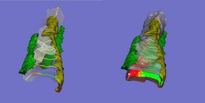
Data Analysis and Visualization Environment (DAVE) is our primary 3D visualization tool. DAVE help and some DAVE images are viewable online.

Simulation

analyze_simulation.pl

This program takes one or more outputs of a simulation (e.g. output of run1 or run2) For each z slice (time point) in each output: blurs it with a psf, pulls out the in-focus slice. Then calculates total concentration CHANGE (relative to time 0) as a function of distance from the calcium entry site (assumed to be the brightest point over all time after blurring). This is written to a file with the same root as the input simulation, but with a .xy extension. This can be viewed with xmgrace, or read into matlab (readxmgr) and visualized with acurves().

Assumes simulation was at 100 nm resolution. Uses a fixed psf with 300x300x150 nm voxels. Several scale factors are applied, so comparisons of magnitudes between files are not valid (but comparisons between time pts from the same file are fine).

analyze_simulation.pl [options] sim.i2i [additional input files]

options: -zrange=#:#:# startz stopz dz, inclusive, zero indexed. default is all z slices (i.e., all time pts). -verbose print out extra into to stderr as it goes along -keepfiles keep all intermediate files. may take lots of space!

examples: analyze_simulation.pl -verbose -zrange=0:10:1 run1_cafl.i2i > & sim.out

       xmgrace run1_cafl.xy

matlab: data = readxmgr('run1_cafl.xy'); acurves(data);

analyze_simulation.pl -verbose run1_cafl.i2i run1_ca.i2i > & sim.out

calc_diffusion3.pl

   This program reads in a 2D diffusion tracks and calculates a D for each file (track_\d+.out)
   by fitting a line to the MeanSquaredDisplacement vs time:

MSD(t) = 4Dt (it would be MSD(t) = 4Dt + 2*sigma^2 if there is noise, see ref below).

   so the slope of the line divided by 4 should yield D (even in the case with noise).
   note: Lag intervals overlap one another unless -no_overlap is specified.
   meanD, varD, and standard error of the meanD is printed to stderr.
   note: if -no_overlap is not specified, the standard error of the mean (seD) may not be correct
         since the points aren't independent.

   calc_diffusion3.pl [options]  

-minlag=# if not specified, minlag = 1 -maxlag=# if not specified, maxlag = 1/2 the total time in the first track file analyzed -duration=# rather than analyze each track in its entirety, split it into (non-overlapping) sections of the specified duration (number of time points). -files=file1:...:filen list of filenames to analyze (instead of all track_#.out files)

       -filerange=#:#	only look at files track_#1.out to track_#2.out (inclusive)

-logfit also do the D calculation (via a line fit) in the log-log space (ln (MSD(t) = ln(4D) + ln(t)) -no_overlap

	-print_Ds	print all the Ds calculated, one per line (tracknum D), to stdout.
	-print_wDs	print all the weighted Ds calculated, one per line (tracknum D), to stdout.

-print_graph prints to stdout MSD vs time -notracknum the filename being read does not have tracknumber in it, just autonumber them. -dummy just print some info to stderr -verbose which file is being analyzed printed to stderr

   example:
       calc_diffusion3.pl  -print_graph files=track_1.xy | cull -c -s -1 -2 |xmgrs

# take a 1,000 pt track and analyze it as 10 separate 100 length tracks to see what those Ds look like:

       calc_diffusion3.pl  -print_Ds -print_wDs -files=track_1.xy
       calc_diffusion3.pl  -duration=100 -print_Ds -print_wDs -files=track_1.xy

   see also:

calc_diffusion.pl same program but only operates on one file. calc_diffusion2.pl same program but without the -duration option SingleParticleTracking_DiffusionCoefficients_Saxton.pdf p. 1746 for the algorithm SubdiffusionOfSingleParticleTracks.pdf - p. 4 gives the formula if there is noise in the estimate.

compare_volume_measurements.pl

This program combines data produced by cross_sections_of_voronoi (-vfile) with an analysis of the same image within fiji (via the stereology_lml macro, -sfile). Results printed (on each line there will be sfile data then vfile data) to stdout.

compare_volume_measurements.pl [options] -vfile=filename1.txt -sfile=filename2.txt

options: -print_volumes rather than print entire combined lines, just print volume info in columns. the columns are: region: the region id, this is the same as the pixel value. sarea: the cross-sectional region area as reported by the fiji stereology_lml.txt macro. svolume: the volume estimated by stereology_lml.txt swvolume: the weighted volume estimated by stereology_lml.txt (not really a true volume). true_volume: the true volume of the region (as created by cross_sections_of_voronoi). area: area as reported by cross_sections_of_voronoi volume_from_area another way to estimate volume from area, w/out stereology: ((1/.68)*area)^(3/2) -vprefix=# foreach field printed out, change its name by adding the specified prefix -sprefix=# foreach field printed out, change its name by adding the specified prefix this may be used so that field names become unique (otherwise, eg, there will be two "area" fields and two "volume" fields on each line). -verbose stuff to stderr

examples: cross_sections_of_voronoi -P voronoi.i2i > filename1.txt Fiji Edit->options->conversions - make sure "scale when converting" is NOT checked.

            Plugins-> open i2i -> voronoi.i2i, then Image->type->32, Image->type->16, to get rid of the table lookup
            Plugins->macros->install... install stereology_lml.txt
            Plugins->macros->stereology_lml.txt  -> voronoi_fiji.txt

compare_volume_measurements.pl -vfile=filename1.txt -sfile=voronoi_fiji.txt

# look at volume estimated via stereology (x axis) vs. true volume (y axis): compare_volume_measurements.pl -print_volumes -vfile=filename1.txt -sfile=voronoi_fiji.txt | cull -c -s -3 -5 | xmgrace -free -pipe

# look at volume estimated from area (x axis) vs. true volume (y axis): compare_volume_measurements.pl -print_volumes -vfile=filename1.txt -sfile=voronoi_fiji.txt | cull -c -s -7 -5 | xmgrace -free -pipe

# compare true volume (x axis) to both the stereology estimated volume and the volume from area measurements (y axis): compare_volume_measurements.pl -print_volumes -vfile=filename1.txt -sfile=voronoi_fiji.txt | cull -c -s -5 -3 -7 > tmp.nxy

       xmgrace -nxy tmp.nxy -free

see also: /home/lml/krypton/Corvera/Raz/stereology/README, run_voronoi.pl cross_sections_of_voronoi /home/lml/krypton/packages/fiji/Fiji.app/macros/stereology_lml.txt

filter_beads.pl

Reads in a file produced by makebeads2 (bead.info) and one produced by print_pixel_coords (mask.info). A bead's info is kept only if at least one of its voxels is under the mask. Kept beads are printed to stdout with their original values (bead id, position, etc.). Thus, if you actually mask the bead image (using maski2i) which was produced by makebeads2, this will keep the associated bead info for those beads which have at least one pixel left in the image after masking.

Note: this can only be run on data produced by versions of makebeads2 newer than 2/12/09.

filter_beads.pl bead.info mask.info > filtered_bead.info

options:

 -keepcenter=#		: rather than keep a bead if any of its voxels is under the mask, only keep the bead

if its center is under the mask. # is the scale factor to convert from the original resolution the bead was created at (-S option to makebeads2) and the resolution of the mask. For example: makebeads2 -S 0.005 0.005 0.005 ... > beads.info If you then use a mask at .1 um you would specify -keepcenter=20

 -verbose

Example:

   makebeads2 -v -d 1280 1280 60 -S 0.005 0.005 0.005  -n 300 -i 1 beads300.i2i > bead.info
   maskimage beads300.i2i mask.i2i beads_masked.i2i
       # now want to filter bead.info to leave only beads at least partially under  mask.i2i (i.e., beads with at least one pixel
       # left in beads_masked.i2i)
   print_pixel_coords -2 mask.i2i > mask.info
   filter_beads.pl bead.info mask.info  > filtered_bead.info

# now filtered_bead.info "matches" what is left in beads_masked.i2i

An example where resolution is changed: # voxel coords printed to bead.info by makebeads2 will reflect the new (chres'ed) coords appropriately:

   makebeads2 -v -d 1280 1280 60 -S 0.005 0.005 0.005  -c 0.025 0.025 0.01 -n 300 -i 1 beads.i2i > bead.info

# now actually change the res of the bead image to match:

   chres -S 5 5 2 beads.i2i beads_ch.i2i

# apply the mask to the lower res image. mask must already be at that same resolution:

   maskimage beads_ch.i2i mask_ch.i2i beads_ch_masked.i2i

# get out coords of all pixels in this low res mask:

   print_pixel_coords -2 mask_ch.i2i > mask_ch.info

# now just keep the bead info for beads which are under the mask at this low resolution:

   filter_beads.pl bead.info mask_ch.info  > filtered_bead.info

# now filtered_bead.info "matches" what is left in beads_ch_masked.i2i (I hope!)

See also: makebeads2, print_pixel_coords

graph_xpp2.pl

Reads specified columns of data from an xpp output file. Sends output stdout.

note: time is always the first variable output (i.e., the first column).

usage:

  graph_xpp2.pl [options] output.dat > name1_name2.dat

options:

  -allstates: 	extract all columns of data having to do with channel state. 

This is all the basic data. Other data is derived from this.

  -openstates:		all open states.  cannot be specified with -closedstates.
  -nopen:		sum of all the open states. cannot be used with -closedstates.
  -closedstates:	all closed states. cannot be specified with -openstates.
  -verbose		

example:

  xpp -silent bk.ode    -> output.dat
  graph_xpp.pl -vars=time:name1:name5:name7 output.dat   > xpp_subset.out
  xmgrace -nxy xpp_subset.out

see also:

  graph_xpp.pl

oxygen_krogh.pl

   NOT DONE YET.

   Calculates steady state oxygen levels as a function of distance from a
   blood vessel (see ~/krypton/Corvera/Olga).
   Writes to (rstar,Pstar) columns to stdout; this is the Krogh-Erlang
   equation. Equation 17 of KroghOxygenDiffusionModel1.pdf

   oxygen_krogh.pl [options]

   options:

   see also: oxygen_krogh.c

random_path.pl

Generate a random path (ie, diffusion).

usage:

random_path.pl [options] > track_1.out

options: -D=# diffusion coefficient, default = 1 -length=# pathlength (number of time points). default = 1000 -xy only print x,y rather than t,x,y

-method=oversample|gaussian oversample takes dt size substeps to calculate each 1 time unit step. gaussian just samples into an equivalent Gaussian distribution once for each 1 time unit step. default: oversample. gaussian option not tested yet... -dt=# substep time interval, default = .001 (only used if -method=oversample). -seed=# so random numbers are the same from run to run (only if -method=oversample)

note: using the default random number generator which is probably not great.

see also: run_random_path.pl calls random_path.pl to generate lots of paths. calc_diffusion3.pl can analyze these paths ~/krypton/diffusion/mytracks/

readbeads.pl

Reads in file produced by makebeads to check to see if sizes and amplitudes are Gaussian and Poission (-G and -P options). Produces _tmpsize and _tmpamp. You may want to use filterbeads.pl prior to using readbeads.pl. You can read these into xmgrace and then create histograms if so desired.

readbeads.pl makebeads.out

-skipzero skip values which are zero -outer put outer diameter (rather than "size") into _tmpsize. If makebeads used the -g option, then size always equals 1. outer should be the gaussian mean + 1/2 shell width. -rpts=# also prints out _coords.rpts file of coordinates of center of beads. This can be read in by addlines. Can also be read by pt_distances. # is a scale factor to divide by to get the new coordinates (so you can compare these to a lower resolution image). Set # to 1 if you don't want to scale the values. Note: coords are truncated an integer value (new = integer(old/# + 1)). skipzero command doesn't affect this option. note: if more than 1 point has the same new coordinates, then the w value for each duplicate point is 1 higher than the previous value (e..g, if -w=-10, then the first (5,6,3) has a w = -10, next has a value -9, next -8, etc. note: this also causes coords to be converted from 0-indexed (makebeads2 output) to 1-indexed (play assumes this for rpts files). -dontrescalez: when using -rpts=#, don't rescale the z coord -twod ignore z dimension when printing rpts file (still must specify -rpts option). -w=# in rpts file, set w to specified number, default = -1000 -amp use the amplitude of the bead for the w value in rpts file output

See also: filterbeads.pl, makebeads2, objs2dist121.pl, print_pixel_coords, filter_beads.pl

run_random_path.pl

Generate lots of random paths files (ie, diffusion) by calling random_path.pl multiple times..

usage:

run_random_path.pl [options]

options: -seed=# so random numbers are the same from run to run -D=# diffusion coefficient, default = 1 -length=# pathlength (number of time points). default = 1000 -xy only print x,y rather than t,x,y -numpaths=# default = 10 paths -rootname=string default: track_ (so files will be called track_#.out) -verbose stuff to stderr

note: using the default random number generator which is probably not great.

see also: random_path.pl calc_diffusion3.pl

run_voronoi2.pl

This script calls cross_sections_of_voronoi many times, and produces an image and output text file from each run.

run_voronoi2.pl [options]

options:
  -num=#	number of times to run. default = 10
  -D=#		-D option to cross_sections_of_voronoi, average diameter, default = 150
  -dummy	don't do anything, just echo to stderr what would be done

voronoi_vs_fiji.pl

compare the true volumes of voronoi regions (as reported by cross_sections_of_voronoi, e.g. voronoi_D170_0001_g0_G250_volume.txt) to those calculated within fiji using stereology_lml.txt (e.g., voronoi_D170_0001.txt)

Graphs volume (x) vs predicted volume (y) (or prints to stdout if -stdout is specified)

note: if looking at weighted volumes (eg, in weighted/ ), the individuals stereologic volumes

     really are meaningless, and you should really just pull out the wmean values from each run.

usage:

 	voronoi_vs_fiji.pl [options]  *volume.txt

options:

 	-vdir=/path/to/directory              location of directory with the output from cross_sections_of_voronoi
                                       (eg. voronoi_D170_0001.txt) default is the current directory

-debug info about all fields on each line printed to stderr

-stdout everything to stdout

-print_avg for each file, just graph mean and std error of the mean (gotten by combining all the data for each file, so may include multiple stereological runs) rather than all data pts note: this will average together the multiple fiji stereology runs which are often in the same *volume.txt file. I think that is ok (but may make the sem look better than it would be from just one run).

-use_wmean just use the mean or wmean stored in the *volume.txt file and compare these values to ??? ... not done yet

examples: cd /storage/big1/lml/Raz/voronoi run_voronoi2.pl -D=170 -num=20 # calls cross_sections_of_voronoi run_voronoi2.pl -D=220 -num=20 # calls cross_sections_of_voronoi Fiji # then run run_stereolgy_voronoi.ijm cd results/

       voronoi_vs_fiji.pl -vdir=..  *D170*volume.txt  # -> voronoi_vs_fij_D170.xmgr
       voronoi_vs_fiji.pl -vdir=.. *D220*volume.txt  # -> voronoi_vs_fij_D220.xmgr

see also: /storage/big1/lml/Raz/voronoi/ - this is where I've done what is shown in the examples above /storage/big1/lml/Raz/voronoi/README, true_vs_predicted.xmgr /home/lml/krypton/Corvera/Raz/stereology/README, run_voronoi.pl, run_voronoi2.pl, compare_volume_measurements.pl, plot_results.pl cross_sections_of_voronoi /home/lml/krypton/packages/fiji/Fiji.app/macros/stereology_lml.txt /home/lml/krypton/packages/fiji/run_stereology.txt analyze_cross_sections_of_voronoi.pl

ball

This program creates an elliptical shell of brightness the specified brightness (-i option) It is used to create test images for Fischer/hmc.

Usage: ball [options] ball.i2i options: -d xdim ydim zdim: dimensions of image, default = (50,100,50) -r x y z: x,y, and z radius in voxels, default = (20.000000,20.000000,20.000000) -s samplerate: number of subsamples in x and z directions per pixel, default = 1 -i intensity: intensity of the ball's shell, default = 100.000000 -b intensity: intensity background voxels, default = 0.000000 -f image: read in the specified image, add the ball image to that (just replaces voxels along the ball's shell with new values). -t thickness: thickness of shell, default = 1.000000

Note: you can call this multiple times to get a shell within a shell

       code in /home/lml/krypton/facil/ball.c 

calc_ca3

1. /home/lml/krypton/bin/calc_ca3

Reads in 4 floating point images (or 4 short int images) as produced by simulation, calculates the difference image deltaca.i2i (as a floating pt image) between the observed free calcium and what would be expected in equilibrium conditions, i.e., [ca]-[predicted_ca], where [predicted_ca]

is kd*[CaFl]/[Fl].  Output concentration in nM. 

All input concentrations should be in nM Each z slice is analyzed separately (i.e., z is assumed to be time).

Usage: calc_ca3 [options] ca.i2i fl.i2i cafl.i2i cafixed.i2i deltaca.i2i options: -k #: kd in uM, default = 1.125000

        -h:		print cumulative histogram for each z slice.
      options for printing graphs of free calcium (not concentration) vs. distance from ca entry location:

the units for the graph are nM*um^3, but 1nM = .6ions/um^3 , so multiply be .6 to get ions

                      (and 1pA = 3,000 ions/msec if you want to convert to pA-msec).
        -c:		print delta calcium (delta from first slice) distance graph for each z slice.
        -n:		normalize delta calcium distance graph for each z slice (so sum of amplitudes = 1),
                      (otherwise when graph spacing is changed, -g option, the height of the graph will change).
        -a:		print absolute calcium, not delta calcium.
                      when this is applied to a uniform image it should produce a 4pi*r*r distribution.
      options for printing graphs of total calcium, i.e. ca+cafl+cafixed (not concentration):
        -C:		print delta total calcium distance graph for each z slice.
        -N:		normalize delta total calcium distance graph for each z slice (so sum of amplitudes = 1).
        -A:		print absolute total calcium, not delta total calcium

-p # #: pixel size in microns in the radial (x) and lengthwise (y) directions, default = 0.10 and 0.10 -P # # #: pixel size in microns in x,y,z directions (rectangular not cylindrical coords), default = ( 0.10, 0.10, 0.10) -r: data is rectangular, not cylindrical coords (-P sets this too) -e x y: 0-indexed coords of calcium entry location (default: x= 0, y = ydim/2)

        -g #:		graph spacing for -c,-C,-n,-N,-a,-A options. defauls is pixel size.
        -s #:         subsample each voxel this number of times in the x (radial) and y (longitudinal) directions,
                      default = 3.  Subsampling only applies to histogram and graph generation, not image generation.
        -z low hi dz: only look at z slices low to hi (0-indexed, inclusive), stepping by dz.
                      The zdim of deltaca.i2i will not change, but skipped slices will be 0.

see also:

   float2int, in matlab: readxmgr, acurves (see ~lml/krypton/JSinger for an example)

source code in ~lml/krypton/Walsh directory.

cellsim

[0]: in main, before MPI_Init()

[0]: in main, after MPI_Init() [0]: /home/lml/krypton/bin/cellsim -h help: unable to parse command: -h

   This program simulates Ca and Na in a cylindrical cell with
   cylindrical symmetry. 
   Note: It is recommended that the stderr output be examined for
         lines with the words: warning, Warning, error, or Error on them.

Usage

   cellsim [options] >& output_datafile

Options controlling the duration of the simulation:

    -time #:       total time to simulate (in sec), default = 0.000000
    -time_rate #:  slow down time, ie take smaller dt steps during simulation.
                   this may be necessary if you are creating a large ca gradient,
                   for example, with -ca_ring or -ca_src options (.5 means 1/2 the dt).
                   The number of iterations needed for convergence is
                   roughly: I= (T*diff)/(dr*dr), where T is time, dr is
                   annulus thickness and diff is diffusion constant.
                   This ignores ion influx,etc.  If you set diffusion rates very
                   small, the iter # calculated will be too small if other stuff
                   is happening, use -time_rate to compensate.

Options controlling the geometry of the model:

    -radius #:     radius of the cell in microns, default = 6.000000
    -rings #:      radius of the cell in rings, default = 60
                   Ring thickness = cell radius/ # of rings.
    -length #:     length of the cell in disks, default = 300
                   Each disk will be the same thickness as a ring.
    -bc Rmax Lmin Lmax:     boundary conditions at maximum radius and minimum and
                   maximum length coordinate (i.e., at the cell ends). These must
                   be the letters I (for infinite) or S (for solid, i.e. no ions go
                   through the membrane). The I option is not always accurate. default: S
    -mask image.i2i: only voxels in image.i2i > 0 are part of the cell.  Use this
                   to specify an arbitrary shape for the cell.
                   Not extensively tested.
    -spacing file: file specifies the spacing along each axis (i.e, size of each voxel).
                   spacing is in nm, one entry per voxel, comment lines ignored (#).
                   The cell direction (X,Y, or Z) must be the first letter on the line.
                   Other characters on the line will be ignored.
                   The number of entries must be < 2000 each direction.
                   Do not specify -rings,-radius,and -length if you use this option.
                   NOTE: the simulation time step goes as (length)^2, where length is
                         the length of the shortest side of all the voxels specified.
                   Any number of entries per line. First R, then D (length). Example:
                   # R direction (10 pixels in this direction, high res at low R)
                   X
                   25 50 75 100 200 300 400 500 600 1000
                   Y (lengthwise) direction (9 pixels in D, very high res in the middle)
                   100 200 300 400 500 540 550 560 1000
                   Use cyl2cart with -spacing option to convert output images to 
                   a uniform spacing. (I haven't added that option yet)
                   Not extensively tested.

Options specifying substances (ions, buffers, compounds) present in the model (10 max):

    -ion name free_concentration D valence: 
                   concentration in mMolar, D in cm^2/sec, valence in absolute value.
                   valence is only used if -ion_src is also specified.
                   concentration is the initial free concentration.
    -buffer name total_concentration D: 
                   concentration in mMolar, D in cm^2/sec.
                   concentration is the initial total concentration (sum of its free and all bound forms).
    -kin bufname ionname boundname onrate offrate D: 
                   kinetics for interaction between bufname and ionname.  Boundname is the
                   name to give the bound pair.  bufname and ionname must have been 
                   specified (with -ion -buffer or -kin options) prior to this option.
                   onrate:in 1/(mMolar*seconds), offrate: in 1/seconds, D: in cm^2/sec  
    -equil_error relerr iter: maximum relative equilibrium error allowed during the 
                   initial calculation of concentrations from the user specified
                   free ion concentrations and total buffer concentrations. 
                   rel_error = ABS((true_kd - calculated_kd)/true_kd). Default = 1e-05
                   This should be small enough unless you have huge buffer
                   concentrations (>100 mM?). iter (an int) is maximum number of iterations
                   to allow during equilibration, max =1 billion, default = 10000000

Options controlling changing conditions:

    -ion_src name current dur lowdisk highdisk lowring highring: 
                   have a current source of the specified ion coming in through the specified rings
                   and numdisk (rings and disks are 0-indexed indices, inclusive).
                   Current is in pA for the specified duration (sec).
                   The current is uniformly divided within the entire specified input volume.
                   All -buffer and -ion options must be specified prior to this.
                   See comments by the -time_rate option.
    -ion_src_file name imagename current duration:
                   Similar to -ion_src, but the specified floating point image is used to
                   scale the input current at each voxel. The total current coming into the 
                   cell is adjusted so that after this per pixel rescaling, it will = "current".
                   -ion_current_trace with op = S, will modify this.
                   Typically do: int2float -M 1 psf.i2i imagename        prior to this.
    -ion_current_trace name filename dt op threshold:  modifies current specified with 
                   the -ion_src or -ion_src_file options.
                   Times which the channel is open (i.e., current flows) is specified in a file.
                   The file is a list of numbers (current or scale), 1 per line, at dt (in sec) intervals.
                   If op = T, currents greater than the specified threshold means channel open, otherwise closed.
                   If op = S, the current as specified with -ion_src is scaled by the number in the list.
                   "threshold" is required but ignored when op = S.  Not extensively tested. 
    -zap_sub name time:
                   At the specified time (in seconds) set the named substance concentration
                   to 0. This does not prevent it from being produced from other reactions.
                   This is useful if an injected "ion" was photons (e.g., photon+caged -> uncaged)
                   and the laser is turned off at the specified time.
    -ion_pump name max_rate n k lowdisk highdisk lowring highring: 
                   have a pump of the specified ion remove ions in the specified rings
                   and numdisks (rings and disks are 0-indexed indices, inclusive).
                   max_rate * [ion]^n / (k^n + [ion]^n),  [ion] and k in mM. max_rate in mM/sec.

max rates are typically given per unit area (8E-7 umoles/(cm^2 sec) for serca pump). If we divide these published numbers by the ring width (typically 100 nm) we can get a rough rate per unit volume. A typical max_rate might be .1 mM/sec (seems high, Polito et al. biophysj, May, 2006 give a rate in terms of []/volume of ~ .001 mM/sec - but they also have a k on the low end, .0001mM, which would compensate some. Shuai & Jung, PNAS, Jan. 21,2003, p. 507 have a max rate of .5 (uM?)/sec.) Typical values for k might be around .0001-.0005 mM. n=2 for serca pump (must be integer)

                   All -buffer and -ion options must be specified prior to this.
    -ion_leak name rate compartment_conc lowdisk highdisk lowring highring: 
                   have a leak of the specified ion introduce ions into the specified rings
                   and numdisks (rings and disks are 0-indexed indices, inclusive).
                   rate * ([compartment_conc] - [ion]),  [] in mM. rate in 1/sec.

Leak rates are usually set to exactly balance the pump at initial ion concentrations. compartment_conc for [ca] in the SR might be around 2 mM. If max_rate = .001mM/sec, k = .0005mM, compart_conc = 2mM, and resting [ca] = 100nM, rate should = .00001923/sec to balance the pump with the leak. note: Leaks INTO the compartment (when [ion]_in_cyto>compartment_conc) are not allowed.

                   All -buffer and -ion options must be specified prior to this.

Options related to output:

    -save name filename type scale dt:
                   Save images of the specified substance (name) to specified file. By default
                   substances are saved in mM.  This will be multiplied by the scale
                   specified here. dt (in sec) is how often to save images.  Type is I
                   (short int, our normal format) or F (floating pt,2x space, more accurate).
                   The first image saved will be prior to any ion current. The last image
                   will always be the end of the simulation. "name" should be as
                   specified with the -ion, -buffer or -kin option.
                   If the image file already exists, new images will postpended to it.
    -save all tag type scale dt:
                   Equivalent to -save for all ions and buffers. Uses default file names,
                   but adds the tag on the end. ions in nM, all else in uM, then times scale.
    -save_flow name rfilename lfilename scale dt:
                   Save flow images of the specified substance (name) to specified files. 
                   rfile is radial flow, lfile is lengthwise flow. Images saved in floating pt. 
                   Flow is in pA (1 pA = 3 molecules/usec) times scale.
                   dt (in sec) is how often to save images.  
    -save_flow all ltag rtag scale dt:
                   Equivalent to -save_flow for all ions and buffers. Uses default file names,
                   but adds the tag on the end. Output same scale as above.
                   NOTE: flow for EACH substance takes 8*(number of voxels) of space.
    -debug #:      set debug level to #. May substantially slow down the simulation.
                   1: extra print statements at init. 2: more testing while running. 3:
    -debug_subvolume #: Normally the total mmoles (in the entire cell) of each saved substance is
                   printed to stderr.  Setting this option will also cause the printing of the
                   total over a subvolume. Subvolume is all y >= # (0-indexed).
                   Example: if a cell has patch region at y=[1,10], setting # to the neck (11) of the
                   patch will let you see how much actually gets out into the main part of the cell.

Options related to MPI (multiprocessor stuff):

    invoke on the wolves as, for example,  mpirun -np 3 -machinefile file_of_machine_names cellsim ...
    -print_proc #:   only print output from the specified process (0 indexed).
                  Some output (eg, Total mmoles of ions, etc) are only valid for process 0.
    -overlap #:   overlap neighboring regions by the specified number of voxels (default = 50)
                  This will also be the number of iterations between necessary synchronization.
    -debug_mpi #:  print MPI info. Execute MPI dummy stubs if MPI NOT present (eg, under Windows,SGI).
                  This version of the executable does NOT use MPI.
    -debug_mpi_proc rank numproc:  set dummy rank and number of processes. use only if MPI NOT present!

EXAMPLES ./cellsim -time .0010 -time_rate .5 -length 200 -rings 40 -radius 1 \

       -ion Ca 100E-6 2.5E-6 2 -buffer Fluo3 .050 2.5E-7 -buffer Buf .230 1E-14  \
       -kin Fluo3 Ca CaFl 8E4 90 2.5E-7 -kin Buf Ca CaBuf 1E5 100 1E-14        \
       -ion_src Ca 1 .00105 99 102 0 3 \
       -save all _run1 I 1 .0001 >& cellsim_run1.out

Simulate for 100msec saving images every msec. 1 pA comes in the the pattern as specified by psf_float.i2i for 10 msec. The current is then modulated by values in current.txt which are one value per line, dt of 1 msec between them. Cell shape in mask.i2i. Voxel sizes in spacing.txt ./cellsim -time .100 -time_rate .5 -spacing spacing.txt -mask mask.i2i \

       -ion Ca 100E-6 2.5E-6 2 -buffer Fluo3 .050 2.5E-7 -buffer Buf .230 1E-14  \
       -kin Fluo3 Ca CaFl 8E4 90 2.5E-7 -kin Buf Ca CaBuf 1E5 100 1E-14        \
       -ion_src_file Ca psf_float.i2i 1 .010 \
       -ion_current_trace Ca current.txt .001 S 999 \
       -save CaFl cafl.i2i I 1000 .001 -save Ca ca.i2i I 1E6 .001 \
       -save_flow Ca ca_radial_float.i2i ca_long_float.i2i 1 .001 >& cellsim.out 

SEE ALSO

      ~lml/vision/bin/float2int                    (convert a floating point image to standard SHORT INT format)
      ~lml/vision/bin/int2float		      (convert normal image to floating point)
      ~lml/vision/bin/playexact                    (to display a floating point image)
      ~lml/invitro/Kargacin/changeheader           (change header of floating point image)
      ~lml/vision/bin/cyl2cart                     (convert from cylindrical to cartesian coords)
      ~lml/vision/bin/nadiffl7                     (many more options, but only 1 ion and 2 buffers)
      ~lml/vision/bin/diffuse2                     (simple Gaussian spot diffusion program)
      ~lml/invitro/Kargacin/iplot                  (3D graph of a 2D image, intensity -> height)
      ~lml/invitro/Kargacin/blur4D_dFoverF         (blur with psf, calculate dFoverF)
      ~lml/invitro/Kargacin/diffusion_limited_binding  (simulate diffusion limited binding)
      ~lml/invitro/Kargacin/spot_diffusion         (simulate diffusion from a spot)
      ~lml/vision/facil/printvals                  (print image values, calculate dFoverF)
      ~lml/vision/JSinger/src/channel              (steady state based upon Neher paper)

cellsimL

[0]: in main, before MPI_Init()

[0]: in main, after MPI_Init() [0]: /home/lml/krypton/bin/cellsimL -h help: unable to parse command: -h

   This program simulates Ca and Na in a cylindrical cell with
   cylindrical symmetry. 
   Note: It is recommended that the stderr output be examined for
         lines with the words: warning, Warning, error, or Error on them.

Usage

   cellsim [options] >& output_datafile

Options controlling the duration of the simulation:

    -time #:       total time to simulate (in sec), default = 0.000000
    -time_rate #:  slow down time, ie take smaller dt steps during simulation.
                   this may be necessary if you are creating a large ca gradient,
                   for example, with -ca_ring or -ca_src options (.5 means 1/2 the dt).
                   The number of iterations needed for convergence is
                   roughly: I= (T*diff)/(dr*dr), where T is time, dr is
                   annulus thickness and diff is diffusion constant.
                   This ignores ion influx,etc.  If you set diffusion rates very
                   small, the iter # calculated will be too small if other stuff
                   is happening, use -time_rate to compensate.

Options controlling the geometry of the model:

    -radius #:     radius of the cell in microns, default = 6.000000
    -rings #:      radius of the cell in rings, default = 60
                   Ring thickness = cell radius/ # of rings.
    -length #:     length of the cell in disks, default = 300
                   Each disk will be the same thickness as a ring.
    -bc Rmax Lmin Lmax:     boundary conditions at maximum radius and minimum and
                   maximum length coordinate (i.e., at the cell ends). These must
                   be the letters I (for infinite) or S (for solid, i.e. no ions go
                   through the membrane). The I option is not always accurate. default: S
    -mask image.i2i: only voxels in image.i2i > 0 are part of the cell.  Use this
                   to specify an arbitrary shape for the cell.
                   Not extensively tested.
    -spacing file: file specifies the spacing along each axis (i.e, size of each voxel).
                   spacing is in nm, one entry per voxel, comment lines ignored (#).
                   The cell direction (X,Y, or Z) must be the first letter on the line.
                   Other characters on the line will be ignored.
                   The number of entries must be < 2000 each direction.
                   Do not specify -rings,-radius,and -length if you use this option.
                   NOTE: the simulation time step goes as (length)^2, where length is
                         the length of the shortest side of all the voxels specified.
                   Any number of entries per line. First R, then D (length). Example:
                   # R direction (10 pixels in this direction, high res at low R)
                   X
                   25 50 75 100 200 300 400 500 600 1000
                   Y (lengthwise) direction (9 pixels in D, very high res in the middle)
                   100 200 300 400 500 540 550 560 1000
                   Use cyl2cart with -spacing option to convert output images to 
                   a uniform spacing. (I haven't added that option yet)
                   Not extensively tested.

Options specifying substances (ions, buffers, compounds) present in the model (10 max):

    -ion name free_concentration D valence: 
                   concentration in mMolar, D in cm^2/sec, valence in absolute value.
                   valence is only used if -ion_src is also specified.
                   concentration is the initial free concentration.
    -buffer name total_concentration D: 
                   concentration in mMolar, D in cm^2/sec.
                   concentration is the initial total concentration (sum of its free and all bound forms).
    -kin bufname ionname boundname onrate offrate D: 
                   kinetics for interaction between bufname and ionname.  Boundname is the
                   name to give the bound pair.  bufname and ionname must have been 
                   specified (with -ion -buffer or -kin options) prior to this option.
                   onrate:in 1/(mMolar*seconds), offrate: in 1/seconds, D: in cm^2/sec  
    -equil_error relerr iter: maximum relative equilibrium error allowed during the 
                   initial calculation of concentrations from the user specified
                   free ion concentrations and total buffer concentrations. 
                   rel_error = ABS((true_kd - calculated_kd)/true_kd). Default = 1e-05
                   This should be small enough unless you have huge buffer
                   concentrations (>100 mM?). iter (an int) is maximum number of iterations
                   to allow during equilibration, max =1 billion, default = 10000000

Options controlling changing conditions:

    -ion_src name current dur lowdisk highdisk lowring highring: 
                   have a current source of the specified ion coming in through the specified rings
                   and numdisk (rings and disks are 0-indexed indices, inclusive).
                   Current is in pA for the specified duration (sec).
                   The current is uniformly divided within the entire specified input volume.
                   All -buffer and -ion options must be specified prior to this.
                   See comments by the -time_rate option.
    -ion_src_file name imagename current duration:
                   Similar to -ion_src, but the specified floating point image is used to
                   scale the input current at each voxel. The total current coming into the 
                   cell is adjusted so that after this per pixel rescaling, it will = "current".
                   -ion_current_trace with op = S, will modify this.
                   Typically do: int2float -M 1 psf.i2i imagename        prior to this.
    -ion_current_trace name filename dt op threshold:  modifies current specified with 
                   the -ion_src or -ion_src_file options.
                   Times which the channel is open (i.e., current flows) is specified in a file.
                   The file is a list of numbers (current or scale), 1 per line, at dt (in sec) intervals.
                   If op = T, currents greater than the specified threshold means channel open, otherwise closed.
                   If op = S, the current as specified with -ion_src is scaled by the number in the list.
                   "threshold" is required but ignored when op = S.  Not extensively tested. 
    -zap_sub name time:
                   At the specified time (in seconds) set the named substance concentration
                   to 0. This does not prevent it from being produced from other reactions.
                   This is useful if an injected "ion" was photons (e.g., photon+caged -> uncaged)
                   and the laser is turned off at the specified time.

Options related to output:

    -save name filename type scale dt:
                   Save images of the specified substance (name) to specified file. By default
                   substances are saved in mM.  This will be multiplied by the scale
                   specified here. dt (in sec) is how often to save images.  Type is I
                   (short int, our normal format) or F (floating pt,2x space, more accurate).
                   The first image saved will be prior to any ion current. The last image
                   will always be the end of the simulation. "name" should be as
                   specified with the -ion, -buffer or -kin option.
                   If the image file already exists, new images will postpended to it.
    -save all tag type scale dt:
                   Equivalent to -save for all ions and buffers. Uses default file names,
                   but adds the tag on the end. ions in nM, all else in uM, then times scale.
    -save_flow name rfilename lfilename scale dt:
                   Save flow images of the specified substance (name) to specified files. 
                   rfile is radial flow, lfile is lengthwise flow. Images saved in floating pt. 
                   Flow is in pA (1 pA = 3 molecules/usec) times scale.
                   dt (in sec) is how often to save images.  
    -save_flow all ltag rtag scale dt:
                   Equivalent to -save_flow for all ions and buffers. Uses default file names,
                   but adds the tag on the end. Output same scale as above.
                   NOTE: flow for EACH substance takes 8*(number of voxels) of space.
    -debug #:      set debug level to #. May substantially slow down the simulation.
                   1: extra print statements at init. 2: more testing while running. 3:
    -debug_subvolume #: Normally the total mmoles (in the entire cell) of each saved substance is
                   printed to stderr.  Setting this option will also cause the printing of the
                   total over a subvolume. Subvolume is all y >= # (0-indexed).
                   Example: if a cell has patch region at y=[1,10], setting # to the neck (11) of the
                   patch will let you see how much actually gets out into the main part of the cell.

Options related to MPI (multiprocessor stuff):

    invoke on the wolves as, for example,  mpirun -np 3 -machinefile file_of_machine_names cellsim ...
    -print_proc #:   only print output from the specified process (0 indexed).
                  Some output (eg, Total mmoles of ions, etc) are only valid for process 0.
    -overlap #:   overlap neighboring regions by the specified number of voxels (default = 50)
                  This will also be the number of iterations between necessary synchronization.
    -debug_mpi #:  print MPI info. Execute MPI dummy stubs if MPI NOT present (eg, under Windows,SGI).
                  This version of the executable does NOT use MPI.
    -debug_mpi_proc rank numproc:  set dummy rank and number of processes. use only if MPI NOT present!

EXAMPLES ./cellsim -time .0010 -time_rate .5 -length 200 -rings 40 -radius 1 \

       -ion Ca 100E-6 2.5E-6 2 -buffer Fluo3 .050 2.5E-7 -buffer Buf .230 1E-14  \
       -kin Fluo3 Ca CaFl 8E4 90 2.5E-7 -kin Buf Ca CaBuf 1E5 100 1E-14        \
       -ion_src Ca 1 .00105 99 102 0 3 \
       -save all _run1 I 1 .0001 >& cellsim_run1.out

Simulate for 100msec saving images every msec. 1 pA comes in the the pattern as specified by psf_float.i2i for 10 msec. The current is then modulated by values in current.txt which are one value per line, dt of 1 msec between them. Cell shape in mask.i2i. Voxel sizes in spacing.txt ./cellsim -time .100 -time_rate .5 -spacing spacing.txt -mask mask.i2i \

       -ion Ca 100E-6 2.5E-6 2 -buffer Fluo3 .050 2.5E-7 -buffer Buf .230 1E-14  \
       -kin Fluo3 Ca CaFl 8E4 90 2.5E-7 -kin Buf Ca CaBuf 1E5 100 1E-14        \
       -ion_src_file Ca psf_float.i2i 1 .010 \
       -ion_current_trace Ca current.txt .001 S 999 \
       -save CaFl cafl.i2i I 1000 .001 -save Ca ca.i2i I 1E6 .001 \
       -save_flow Ca ca_radial_float.i2i ca_long_float.i2i 1 .001 >& cellsim.out 

SEE ALSO

      ~lml/vision/bin/float2int                    (convert a floating point image to standard SHORT INT format)
      ~lml/vision/bin/int2float		      (convert normal image to floating point)
      ~lml/vision/bin/playexact                    (to display a floating point image)
      ~lml/invitro/Kargacin/changeheader           (change header of floating point image)
      ~lml/vision/bin/cyl2cart                     (convert from cylindrical to cartesian coords)
      ~lml/vision/bin/nadiffl7                     (many more options, but only 1 ion and 2 buffers)
      ~lml/vision/bin/diffuse2                     (simple Gaussian spot diffusion program)
      ~lml/invitro/Kargacin/iplot                  (3D graph of a 2D image, intensity -> height)
      ~lml/invitro/Kargacin/blur4D_dFoverF         (blur with psf, calculate dFoverF)
      ~lml/invitro/Kargacin/diffusion_limited_binding  (simulate diffusion limited binding)
      ~lml/invitro/Kargacin/spot_diffusion         (simulate diffusion from a spot)
      ~lml/vision/facil/printvals                  (print image values, calculate dFoverF)
      ~lml/vision/JSinger/src/channel              (steady state based upon Neher paper)

channel_current2

channel_current2: like channel_current, but looks at [ca] over time at each BK (not just max [ca]). From that, it calculates the max BK current. Channel_current adds the max [ca] that each BK voxel sees from each voxel in a Ryr cluster, to get the max [ca] that BK pixel sees. But the max [ca] could occur at different times since the Ryr cluster has a spatial extent. Experimental.

Calculates the current which would be produced when each object in Ryr_image.i2i releases calcium which activates nearby BK channels in BK_image.i2i. Produces a histogram of these output currents. The input images should have each pixel in an object having the object id as its value. These images can be produced with "countobjs -Q" or "objs_via_ascent" note: a one pixel border around the image is ignored (added 12/8/09). This may take about one-half hour to run.

Usage: channel_current [options] -f filename Ryr_image.i2i BK_image.i2i > im1_im2.hist Options: -f filename resting: file containing [ca], in nM, as a function of distance and time. Right now this is assumed to have 20 nm spacing and entries every msec. See /home/lml/krypton/Zhuge/STIC/simulations/run32.ca as an example "resting" is the resting [ca], in nM, for the cell. It will we subtracted from the other [ca] values to produce a "delta" [ca] which gets scaled linearly by Ryr intensity. The spark current used to produce this (see -C) should be roughly in the range expected for Ryr_image.i2i, since all delta [ca] is linearly extrapolated. All distances > largest distance in filename will have their [ca] set to the [ca] at the largest distance in filename. note: Only the [ca] values at y == 1 are used. Is this what should be used? -u #: voltage (mV). BK conductance is a function of voltage. default = -80.000000 -U low delta hi: voltages from low to hi by delta. Max is 20 voltages -r #: resolution (binsize) for output histogram in femtoAmps, default = 1000.000000 -R #: reveral potential of BK channel in mV, default = -80.000000

  distances:

-w # # #: x,y, zweights for pixel distances (ie, pixel size), default = 1 for each. -p #: pixel size in nm (i.e., what 1 means in -w option), default = 80.000000 -m # : maxdistance (in units used for -w, i.e., pixels) to look for the closest pixel, default = 10.000000

  which pixels or clusters to include:

-t # #: image1 and image2 thresholds, pixels > # are above threshold, default = 0. -e lowx lowy lowz hix hiy hiz: only look at voxels within this extent (subvolume), 1-indexed, inclusive. -s minsize maxsize: only look at objects in Ryr_image.i2i within the size range (inclusive, in voxels) max size allowed = 100000 -S minsize maxsize: only look at objects in BK_image.i2i within the size range (inclusive, in voxels) -i miniod maxiod: only look at objects in Ryr_image.i2i within the iod range (inclusive. use -d also.) -I miniod maxiod: only look at objects in BK_image.i2i within the iod range (inclusive. use -D also.)

  scale factors:

-d Ryrimage1d.i2i #: the original intensity image for Ryr_image (since Ryr_image has pixel values as id numbers) # is the number of Ryrimage1d.i2i intensity units required to produce spark current used in the calcium simulation (which produced the -f filename data). This will scale the [ca] produced by each Ryr voxel. Default = 30000.000000 -D BKimage2d.i2i #: the original intensity image for BK_image (since BK_image has pixel values as id numbers) # is the BKimage2d.i2i intensity from one BK channel. This will scale current produced. Default = 1000.000000 If you want the intensity of each Ryr or BK object to affect the ca release (for Ryr) or number of channels (for BK) , you need to provide the original data by using the -d and -D options. Otherwise all voxels in an object contribute equally (so large objects have more receptors or channels than small ones). -c #: BK single channel conductance in pS, default = 220.0 -C #: peak current (in pAmps) used in the simulation to produce -f filename, default = 1.000000 This is just used for output produced by -v to estimate spark current produced per Ryr cluster.

  miscellaneous:
 	-v: 			verbose. produces list of each Ryr cluster and K current produced to stderr. Other stuff too.

To write this to a separate file do: (channel_current -v ... > stdout.channel) >& stderr.channel

 	-V: 			very verbose

Examples:

cellsim -spacing /home/lml/krypton/Zhuge/STIC/simulations/spacing2.txt .... : produces ca.i2i printvalsL -spacing2.txt -R -t -i ca.i2i > ca.vals kate ca.vals : delete fist comment line

      objs_via_ascent -s 5 100 Ryr.i2i Ryrid.i2i > tmp 

tail tmp : the mean IOD gives an idea of brightness needed to produce current used in cellsim, say 30000

      objs_via_ascent -s 5 100 BK.i2i BKid.i2i > tmp 

tail tmp : the mean IOD gives an idea of brightness of a BK cluster, eg mean= 10000, but assume that's 10 channels

channel_current -f ca.vals -w 1 1 3 -d Ryr.i2i 30000 -D BK.i2i 1000 Ryrid.i2i Bkid.i2i > ryr_bk.info cull -s -c -1 -4 < ryr_bk.info |xmgrace -source stdin See also: closest_object closest_voxel objs_via_ascent /home/lml/krypton/Zhuge/BKandRyr/graph.pl,match.pl graph_channel_current.pl, test_channel_current, /home/lml/krypton/Zhuge/STIC/simulations/run32 /home/lml/krypton/Zhuge/BKandRyr/analysis6/cluster_distances.pl, plot_mean_sd_curve.pl /home/lml/krypton/Zhuge/xpp/ASM15.ode Bugs:

Source code in ~krypton/lml/facil

# Popen is monotonic as it should be.

must provide -f cafilename

cluster

Drops random Ryr receptors into a world. Then calculates how many clusters and their sizes get produced. Currently the "world" default size is (2um)^3. (see -wsize) The origin of this world is in it's center (so it goes from -1um to +1 um in each direction by default). A histogram of cluster sizes is printed to stdout.

Usage: cluster [options] Options: distance options: -eucliddist: calculate a Euclidean distance (same in x,y,z directions). This is the default. (use -cdist option to set the nearby distance for this). -absdist: rather than calculate a real distance, calculate max(ABS(dx),ABS(dy),ABS(dz)) - for speed (use -cdist to set the nearby distance for this.) -psfdist x y z: distance (in um) a pt can be in the x, y, and z directions and be considered nearby. Does not use -cdist. To approximate a psf you might specify .2 .2 .6

      -cdist #:         how close (in um) two receptors must be to cluster, default = 0.500000

other options:

      -2D:		  do a 2D simulation (x and y), not a 3D simulation

-cylinder inner outer: only place Ryr within a cylinder (e.g., plasma membrane) with specified

                        inner and outer radius (in um). The cylinder has its length the entire y dimension.

Only the parts of the cylinder which fit in the world (-wsize) are used. -wsize x y z: the width of the world (in um) in the x, y, and z directions (default = 2.0,2.0,2.0) -psize x y z: pixel width (in um) in the x, y, and z directions (default = 0.1,0.1,0.1)

      -numryr #:        number of Ryr receptors to drop, default = 1000

-mindist #: when placing Ryr receptors, keep this minimum distance (in um) between them. -randstart #: start the random number generator with # as the seed. So runs can be reproduced. -image name.i2i write out an image of the Ryr receptors. Can then use blur3d to create a realistic microscope image, and countobjs to analyze it and compare to real data. diagnostics:

      -debug:           turn on debugging
      -verbose:         be a bit more verbose
      -h:   print this help
      -H:   print this help
      -help:   print this help

Examples:

Source code in ~krypton/lml/Zhuge/Ryr_clusters

/home/lml/krypton/bin/cluster -h 

diffusion_limited_binding

unknown option h

Prints out distance (um) and concentration (particles/cm^3) at that distance a slab volume of initial uniform concentration (1 particle/cm^3)which has a ligand binding to a plane at x = 0. This is diffusion limited binding. See my notes of 10/20/98.

Usage: diffusion_limited_binding [options] options: -D #: diffusion (cm^2/msec), default = 2.2E-09 -t t1 t2: start and stop time to simulate (msec), default = 0.000000 1000.000000 set both numbers equal if you only want one time point. -x x1 x2: start and stop distances to print (um), default = 0.000000 10.000000 set both number equal if you only want one position -L #: thickness of slab volume (um), default = 10.000000 -T #: number of samples in t, default = 10 -X #: number of samples in x, default = 1000 -h: print this help message. -F: print out time (msec) and flux (particles/cm^2-msec) at x = 0 (i.e., rate molecules binding to x=0 surface). I've made flux towards lower x positive (normally it would be negative). -B: print out time (msec) and total # of particles/cm^2 bound at x = 0 (i.e., brightness of surface). Integral of flux from t1 = 0 regardless of -t option setting. -s: don't print out concentration as a function of x (i.e, the entire slab)

ellipse

This program creates an elliptical cell, cell length is in the y direction. It is used to model a squashed cell, and see how different it looks after blurring than a cylindrical cell

Usage: ellipse [options] ellipse.i2i options: -d xdim ydim zdim: dimensions of image, default = (50,100,50) -r xradius zradius: radius (in pixels) in the x and z directions, default (20.000000,20.000000) -s samplerate: number of subsamples in x and z directions per pixel, default = 1 -i intensity: intensity inside the ellipse, default = 100.000000

em

Creates (or reads in) a HMM and then generates random data from it (each model is a poisson process, with the j_th model having a lambda = 10*j). Then attempts to use an EM algorithm to estimate the original model. This is a way for me to learn how to implement the EM algorithm.

Usage: em [options] options: -s #: number of states, default = 2. Must specify -t and -p after this. -t # # # ... #: state transition probabilities. If there are S states (e.g., -s #)

                        order: T[1][1], T[1][2], ... T[1][S], T[2][1] ... T[S][S] if there are S states),
                        where T[i][j] is the probability of a transition from state i to state j.

-p # # # ... #: prior probabilities of states (S entries if there are S states) -P #: which prior estimate to use for the pdf of the data (ie., estimate of Poisson process) 1 = uniform, 2 = delta, 3 = uniform+delta, 4 = peice of observed data histogram (default) 5 = true pdf (Poisson) -n #: number of data points to simulate, default = 100 -m #: maximum number of iterations to perform, default = 20

        -truetrans:	use the true transition probabilities as the initial guess (default = uniform)
        -trueprior:	use the true prior probabilities as the initial prior guess (default = uniform)

-findstates: also find (and print) the estimate of the states at each time point. -v: verbose. print more info to stderr. -V: print some more info. Some printouts only occur if # data pts is < 1000

Source code in /home/lml/krypton/facil/em.cc See also: ~/krypton/facil/transpose.pl to print out selected lines from the output file

          ~/krypton/matlab/netlab: has EM routines
          ~/krypton/matlab/bayes/BNT/HMM: has HMM and EM routines
/home/lml/krypton/bin/em -h 

Statistics

cluster_distances.pl

Takes output from channel_current2 (after 11/24/09) and pulls out statistics about
mean distance to each BK cluster.  Then produces average stats from all the files
analyzed. Output to stdout.

usage:

 -files:file1:file2:...:filen	      which files to analyze. Defaults are files named 2_*.currents in cwd.
 -numBKvsProb			      also prints numBK vs prob data suitable for xmgrace

example:
 (channel_current2  .... > file.channel_current) >& file1.currents
 (channel_current2  .... > file2.channel_current) >& file2.currents
 cluster_distances.pl -numBKvsProb -files=file1.currents:file2.currents > avg_distances.txt
 fgrep -v clusters avg_distances.txt |xmgrace -pipe

note: mean distances to clusters are not always increasing (e.g., mean distance to 10th
      cluster could be SMALLER than the mean distance to the 9th cluster).  I think this
      has to do with limiting my maximum distance (see comments in this file).

see also:
 channel_current2
 /home/lml/krypton/Zhuge/BKandRyr/analysis6/run12
 /home/lml/krypton/Huang/Kth_pt.m
 p. 637 of Cressie. 

coloc.pl

calls coloc3way with a bunch of different thresholds. Creates an output file which can be graphed with VennDiagram.m.

coloc.pl im1.i2i im2.i2i im3.i2i > out.coloc3way

options: -time_vs_thresh just generate a file which shows which times correspond to which thresholds. images can be dummy names.

-t1=#:#:# threshold one should go from # to # by #. default = 800:1200:50 -t2=#:#:# threshold two should go from # to # by #. default = 800:1200:50 -t3=#:#:# threshold three should go from # to # by #. default = 2000:4000:200

	-numthresh=#1:#2:#3   ignore the third number in the -t1, -t2, and -t3 options (or in the default) and instead calculate a 

threshold step size so that #1 thresholds are applied to im1.i2i (dat image) #2 thresholds are applied to im2.i2i (ctx image), #3 thresholds are applied to im3.i2i (rin image). e.g., -numthresh=5:10:10 will apply 5 different thresholds to im1.i2i, and 10 thresholds to im2.i2i and im3.i2i. Using this option lets me insure that each call to coloc.pl will produce exactly the same number of data points; this may make the statistical comparison between cells easier.

-Melikian=file in addition to creating output for VennDiagram, create text file with the coloc percentages Dr. Melikian is interested in. Graph via xmgr -nxy. See header in file for coloc info. For this to work the three image files MUST be specified in the order 405 594 488 (i.e., rin.i2i ctx.i2i dat.i2i) -Melikian2=file Same as -Melikian, but dat (488) is image 1, ctx (594) image 2, and rin (405) image 3 -area=file.xyr also print out Melikian data as xyr where r is proportional to the number of pixels involved (i.e., the denominator used when calculating the percent colocalized). prints to "file.xyr". Must also specify either -Melikian or -Melikian2 xmgrace -graphtype fixed -settype xyr file.xyr -matlab=file:# like -area but as columns so easy to read into matlab: t p1 n1 p2 n2 p3 n3 p4 n4 # is the max n value (ie, all n values are scaled so the max over n1,n2,n3,n4 is #). Since p1,p2,p3,p4 are percent, # is typically set to a small part of that, e.g. .05. If # is negative then abs(#) is just used as a scale factor (so -1 would just keep the n values as the number of voxels). Graph in matlab with line width of 2*n1: matlab # import data=(tdim,9) >> lowy = data(:,2) - data(:,3); hiy = data(:,2) + data(:,3); x = data(:,1); >> area(x,hiy,'FaceColor',[1 0 0],'EdgeColor','r','LineWidth',1); hold on; >> area(x,lowy,'FaceColor',[1 1 1],'EdgeColor','r','LineWidth',1); Must also specify -Melikian or -Melikian2.

-debug -verbose

example:

coloc.pl im1.i2i im2.i2i im3.i2i > coloc.data coloc.pl -time_vs_thresh im1.i2i im2.i2i im3.i2i > coloc.times matlab >> VennDiagram('coloc.data','percent') # and manually look at coloc.times while doing this to convert times to thresholds.

see also: ~/krypton/packages/fiji/Fiji.app/plugins/jacob_.jar - more traditional colocalization measures coloc_tseries2 colocalizeL

probcircle.pl

 given a sphere of diameter D, what is the prob of oberving a disk of radius r when a random plane intersects it?
 prints to stdout: r  prob(r) 1/prob(r)

 usage: 
     probcircle.pl [options] 

 options:

-D=# default = 1 -just_prob don't print the third column

 examples:
     probcircle.pl | xmgrace -free -pipe -nxy -

 see also: p. 249 stereology_book.pdf

/home/lml/krypton/packages/fiji/stereology_lml.template /home/lml/krypton/Corvera/Raz/stereology/plot_results.pl /home/lml/krypton/facil/cross_sections_of_sphere

compare2dist

This program calculates whether two amplitude distributions are the same. It was written to examine Rhonghua's STOCS data to determine whether the increase in observed STOC frequency could be explained by an increase in STOC amplitude (since then more events above threshold would be observed). datafile2 should be the one with larger amplitudes (so we hypothesize it has fewer missing events if it is just a version of datafile1 shifted higher). It will get shifted down by a range of shifts (-s option) and compared with datafile1. This routine also compares the temporal interarrival time distribution of each datafile with that predicted by a poisson process and with the other datafile; the temporal calculations ignore all missing data issues and shifting issues for now.

This program reads data in the form:

   time calcium prior_baseline post_baseline amplitude 
      where the values are
      time:            time of STOC
      calcium:         SR calcium level
      prior_baseline:  amplitude just prior to STOC
      post_baseline:   amplitude just after STOC
      amplitude:       amplitude amplitude of STOC (not relative to baseline)

Data is expected to already be sorted by time (smallest to largest). comment lines must begin with a #

Usage: compare2dist [options] datafile1 datafile2 options: -t #: only include data with an amplitude > #. The default is to assume a 0 threshold. If you have acquired the data using some thresholding criterium (eg, only peaks above 10picoamps are counted) then you should provide that number here, even if all your data is above this (ie, you've applied the threshold in your identification phase). This is because we need to know it when we shift amplitudes of the second distribution to see if it could match the first distribution. -b: subtract average baseline from amplitude prior to use (ie, prior to any thresholding or intensity shifting of data). -s delta max: shift datafile2 amplitudes down by a maximum of max, in increments of delta, to see if it will then match datafile1. -p #: our guess of the percentage of data missing from datafile2 because it was below our threshold/detection criteria (a # from 0 to 1). This plus the amount of datafile2 shifted below threshold determines our estimate of the amount of data missing from the shifted datafile2 and the unshifted datafile1. The larger this number is, the more likely the two curves will appear similar (since differences in actual data examined will be proportionally smaller differences, and we are assuming all missing data matches exactly, but see -m below). Default = 0.000000

 	   -m:		assume all missing data maximally MISmatches, this would probably be

a worst case scenario, so that if the KS statistic says the distributions could be the same even with the -m option, its probably true. But I'm not certain of this, since it really depends how this affects the relative spacing between the cumulative distributions. I'd have to think about it some more.

see also:test_distr, poisson This code is in ~lml/vision/Rhonghua/STOCS

#/home/lml/krypton/bin/compare2dist 

compare2gaussian

incorrect command line, need 1 data files. This program calculates whether a given set of data could be samples from a known mixture of Gaussians. datafile should have one data point per line. comment lines begin with #. Output statistics to stdout.

Usage: compare2gaussian [options] datafile options:

   	   -t #:	only include data with an amplitude > #. The default is to include all data.

-g # amp1 mean1 sd1 ... : The Gaussian mixture model the data should be compared against (using a KS statistic). # is the number of Gaussians, this is followed by the amplitude, mean, and sd of each Gaussian. The default is one Gaussian with mean = 0 and sd = 1. You can get these values using the fitgaussians2 program. -v: verbose. Also prints the observed (first) and theoretical (second) curves to stdout. -T: test. runs through x = 0 to 10 and prints out cumulative prob. exits.

See Also: fitgaussians2, fit2gaussians, fit3gaussians

Source code is in ~lml/krypton/Lefkowitz

#/home/lml/krypton/bin/compare2gaussian 

compare_dist2

This program calculates whether two distributions are the same using chi-square test (unless -k). It was written to examine the distribution of sizes of Ryanodine Receptor objects to determine if they are randomly distributed. datafile1 should be the reference data (gotten from many simulations or from a theoretical formula), datafile2 should be the real data (max number of data values = 100000).

This program reads data which is just a list of sizes of objects seen (one per line). Comment lines must begin with a # Floating pt numbers are truncated to integers for bin number (max bin number = 50000).

Usage: compare_dist2 [options] datafile1 datafile2 options: -k perform K-S test instead (I'm not certain the numbins I use to calculate this is correct). -a also print the histograms produced -b also print the normalized histograms (total count datafile2 scaled to the same count as in datafile1, bins with 0 removed), this is only done if -k not specified (ie, only if performing chi-square test). -c also print the cumulative prob distributions (only done if -k also specified) -r # #: only analyze sizes within the specified range (inclusive) -m #: cap the maximum number of counts for any size in datafile1 to # -M #: cap the maximum number of counts for any size in datafile2 to # -z: for chi-square keep zero entry bins (chi square only correct if this option is NOT used) so why is this option here? if you just really want to use this program to do histogram normalization (-b), and don't care about the stat. xmgrace running avg will produce strange results if you don't use -z, ie, if data not equally spaced. -v verbose -V very verbose example:

      create a simulated distribution and compare it with real restored data (real_ryrr.i2i, run5 does this 100 times):
  cluster -wsize 10 43 25 -cylinder 0.001 3 -psize 0.08 0.08 0.25 -mindist 0.030 -numryr 500 -image ryr.i2i
  blur3d -S 40000 -P ryr.i2i psf.i2i ryr_b.i2i
  noise -c RCA ryr_b.i2i ryr_bn.i2i
  setenv myloc /home/lml/krypton/Zhuge/Ryr_clusters 
  setenv eprloc /storage/big1/epr/queues 
  echo "  /storage/big1/epr/run_epr -V -log -NSC 4 -sm 1e-05 -it 5000 -sc 0.025 -co 0.001

-psf ${myloc}/psf.i2i ${myloc}/ryr_bn.i2i ${myloc}/ryr_bnr.i2i " > /storage/big1/epr/queues/standard/lml.0

  while (1==1)  if ( ( ! -e ${eprloc}/standard/lml.0 ) && ( ! -e ${eprloc}/running/lml.0 ) ) then break endif sleep 60s end 
  countobjs -k -s 5 300 -t 4500 4500 sim_ryr.objs ryr_bnr.i2i
  cull -s -c -2 < sim_ryr.objs > sim_ryr.stats
  countobjs -k -s 5 300 -t 4500 4500 real_ryr.objs real_ryrr.i2i
  cull -s -c -2 < real_ryr.objs > real_ryr.stats
  compare_dist2 -b sim_ryr.stats real_ryr.stats  >& chi_ryr
  compare_dist2 -k -b sim_ryr.stats real_ryr.stats  >& ks_ryr
  tail chi_ryr ks_ryr
  xmgrace chi_ryr; xmgrace ks_ryr

see also: cluster, run5 This code is in /home/lml/krypton/Zhuge/Ryr_clusters/

#/home/lml/krypton/bin/compare_dist2 

correlationL

/home/lml/krypton/bin/correlationL

This program plots intensities from image1 vs intensities from image2. image1 on the x axis, image 2 on the y axis. Intensities in both images are rescaled 0 to the size of the output image (default = 512). The intensity at each pixel in the output image is the number of (image1,image2) voxels with that particular intensity combination. The intent is to be able to look at the output image and get a sense for whether there is a correlation between intensities in the two images. If so, perhaps a least squares line fit should be done to see how well one images correlates with the other, or -s option can be specified. The minimum, maximum, and scale factors are printed to stdout. Version 1.1

Usage: correlation [options] im1.i2i im2.i2i out.i2i options: -d xdim ydim: output dimensions of new image (default = 512,512). -S im1scale im2scale: scale intensities with these scale factors. newval = (intens-min_intens)*scale -B b1 b2: force min_intens (black level) to specified value. newval1 = (intens-b1)*scale1 -i val1 val2: Ignore any voxels in image1 <= val1 and any voxels in image2 <= val2.

-h val1 val2: Ignore any voxels in image1 >= val1 and any voxels in image2 >= val2.

-r: instead of intensities, use the rank order of the intensities. -a: automatically calculate the size of the output image. attempts to make the scale factor = 1. -b: keep the xdim and ydim scale factors the same. -s: calculate Spearman rank-order correlation coefficients. print results to stdout. -z zslice: only examine the specified z slice (the first slice is considered slice 0). note: entire image name is NOT required. note: a - in place of an image name means stdin or stdout.

examples:

    # to apply this to a set of 3D images, using the same scales and size images for easy comparison

correlationL -S s1 s2 -d 512 512 -B 0 0 image1.i2i corr1.i2i (and same for other images)

create_imagesL

This program takes output from many runs of "overlap" and produces two images. One image is a percent colocalization image and the other is a probability image. The overlap program MUST be run via the "many_overlaps" command. The probability calculations are the same as those performed by "probcolocal", but only -n needs to be specified since the other values are automatically extracted from the file produced by "many_overlaps".

The percent image is the percent of voxels above threshold in image1 (as originally specified to "many_overlaps") which overlap with voxels above threshold in image2. A 100 in the output image = 100 percent. The probability of observing as much (or more) overlap as we did due to random chance is the prob.i2i image. Probabilities are mulitplied by 100.

Position along the y-axis (vertical axis) of the image, corresponds to thresholds for image2. The x-axis represents image1 thresholds. The lowest threshold is the bottom left corner. See the first line in your datafile for the range of thresholds this represents. Overlap produces statistics for a range of allowed overlaps. Create_images, by default, chooses an overlap within 1 voxel. If you want to use a different overlap distance use the -o option.

See also: overlap, probcolocal, many_overlaps

Usage: create_images [options] datafile percent.i2i prob.i2i options: -o distance: voxels within this distance count as overlapped. -n number: number of voxels (1000000 default), see probcolocal.

Examples:

  many_overlaps -t 100 1000 100 -T 100 1000 100 alpha_T.i2i beta_T.i2i tmp_output
  create_images -n 363264 tmp_output percent.i2i prob.i2i

Analysis of Points

components.pl

Calculates the number of connected components resolved over a range of point densities.

components.pl [options]

options:

-numpts=low:hi:delta -repeat=# number of times to repeat at each point density -res=# in microns -outfile=name name of output file. otherwise to _tmp. always need write permission in current directory.

convex_hull.pl

This program takes an object outputfile (unless -rptsin or -tripletsin) produced by countobjs (or maskobjs) and finds the minimal spanning tree connecting the center of mass of the objects, and the convex hull. Writes out connections as an rpts file to stdout. It also loops through 20 thresholds for the pts, and prints to stderr some stats about the minimal spanning tree and convex hull of the points above each of these thresholds.

Options can be used to only selected a subset of the objects and to constrain the maximum distance (-maxdist).

It was written with the hope that triplets (maxima in an image which has a cell in the center) will show a pattern in their convex hull area, so that when the threshold rises high enough, only maxima inside the cell will still be present and hence the convex hull will be stable and of much smaller area.

This program requires perl modules Graph::Kruskal and Math::Geometry::Planar, use cpanp to install these:

   yum install perl-CPANPLUS-0.91.3-202.fc16.noarch   - for cpanp
   cpanp -i Graph::Kruskal
   cpanp i Math::Geometry::Planar

usage:

 convex_hull.pl -tripletsin file1.triplets  > file1_mst.rpts

 input options:
    	-dx=#			   spacing in the x direction, default = 1
    	-dy=#			   spacing in the y direction, default = 1
    	-dz=#			   spacing in the z direction, default = 1
    	-rptsin		  	   instead of file1.objs, read file1.rpts where file1.rpts was produced by max2d.

-size1 and -iod1 are ignored when this option is specified.

    	-tripletsin		   instead of file1.objs read in file1.xyi,  triplets of x y and intensity.

 analysis options:
    	-size1=min:max	  	   min and max object size allowed for file1.objs in pixels (inclusive)
    	-iod1=min:max		   min and max object iod allowed for file1.objs (inclusive), or intensity if -tripletsin was specified.
    	-maxdist=#:		:  don't allow connections between pts further apart than this distance (after applying dx, dy, dz spacing factors).

warning: if the distance is too small, then all the pts will not be connected to begin with; this may cause the minimal spanning tree algorithm to fail. default maxdist is 3000

 output options:
    	-addlines		:  output rpts format which addlines is more likely to be happy with (may not work in dave?)
    	-hist			:  calculate histogram of distances (hist[int(dist)]++, where int just truncates to integer). obsolete.
    	-sizehist		:  calculate histogram of object sizes (in voxels) in file1.out. (hist[int(size)]++, where int just 

truncates to integer). If you don't care about distances between two files (ie, only want -sizehist) put the same file name for both files on the command line. obsolete.

    	-rpts=file.rpts	:  put bounding boxes around objects found and lines between closest objects (similar to objs2bb.pl)

display this in dave eg: dave -n 0 -u -I file.i2i file.rpts (use the -n 0 and -u options) note: may not show up in dave until you click on "scale" to force a rescale (or draw?).

    	-jack=max.rpts:#	:  create an rpts file with the maxima in each object displayed as a small jack. 

# controls the size of the jack. 1=1 pixel in size, 2 = 2 pixels, etc. -twod add this (in addition to -jack) if you want 2D jacks rather than 3D jacks.

    	-strlim=#		:  limit length of names of objects in rpts files to # characters.  dave sometimes crashes if the

names are too long.

    	-tyz			:  transpose coords in yz before writing them to the rpts (must specify -rpts option)
    	-color=#		:  for the w value (color) use the specified value (use -P in play to see this as a color). default = none.

if you have no color (no w value), addlines can put one in (-P option in addlines).

 diagnostics:
    	-silent			:   suppress warning messages.
    	-verbose

-debug

example:

 convex_hull2.pl -tripletsin -jack=jack.rpts:5 -addlines -twod -maxdist=100 file1.triplets  > file1_mst.rpts
 addlines2 -P -1 image.i2i file1_mst.rpts - | addlines2 -P -2 - jack.rpts - | reduceima -bin 3 3 -L - -| play -P -1 R  -P -1 G -

see also:

 convex_hull, objs2mst.pl
 objs2bb.pl, objs2dist.pl, objs2dist121.pl, closest_object, closest_voxel, countobjs, maskobjs, objs_via_ascent
 resolve_pts

objs2alldists.pl

Like obs2disp.pl but calculates the distance to ALL the objects (within -maxdist), not just the closest. See ~/krypton/Zhuge/grants/AsthmaRO1/README for 5/27/11 and /home/lml/krypton/Zhuge/BKandRyr/analysis6/run18

  (which did NOT use this).

This program takes 2 object outputfiles produced by countobjs (or maskobjs) and finds the shortest distance from the center of mass of objects in file1.out to the center of mass of objects in file2.out.

If both file arguments are the same (e.g., objs2dist.pl file1.out file1.out >file.dist), you can use this routine to find the distances between objects within an image (an object match with the same id is automatically ignored in this case so objects don't match to themselves). See also the option -skipsame.

(modified from /storage/big1/lml/was_voxel/Corvera/track/objs2bb.pl)

usage:

 objs2alldists.pl file1.out file2.out >file.dist  

options:

 -dx=#			:  spacing in the x direction ,default = 1
 -dy=#			:  spacing in the y direction ,default = 1
 -dz=#			:  spacing in the z direction ,default = 1
 -size1=min:max	:  min and max object size allowed for file 1 in pixels (inclusive)
 -size2=min:max	:  min and max object size allowed for file 2 in pixels (inclusive)
 -iod1=min:max		:  min and max object iod allowed for file 1 (inclusive)
 -iod2=min:max		:  min and max object iod allowed for file 2 (inclusive)
 -maxdist=#:		:  don't allow matches further away than this distance (after applying dx, dy, dz spacing factors).

default maxdist is ~ 3000.

 -hist			:  calculate histogram of distances (hist[int(dist)]++, where int just truncates to integer).
 -sizehist		:  calculate histogram of object sizes (in voxels) in file1.out. (hist[int(size)]++, where int just 

truncates to integer). If you don't care about distances between two files (ie, only want -sizehist) put the same file name for both files on the command line.

 -rpts=file.rpts	:  put bounding boxes around objects found and lines between closest objects (similar to objs2bb.pl)

display this in dave eg: dave -n 0 -u -I file.i2i file.rpts (use the -n 0 and -u options) note: may not show up in dave until you click on "scale" to force a rescale (or draw?).

 -jack=max.rpts:#	:  create an rpts file with the maxima in each object displayed as a small jack. 

# controls the size of the jack. 1=1 pixel in size, 2 = 2 pixels, etc.

 -strlim=#		:  limit length of names of objects in rpts files to # characters.  dave sometimes crashes if the

names are too long.

 -tyz			:  transpose coords in yz before writing them to the rpts (must specify -rpts option)
 -skipsame		:  don't match an object in file1.out to an object with the same id in file2.out

This is set automatically if file1.out = file2.out.

 -silent		:  don't print the distances (sets -hist)
 -simpleprint		:  when printing distances, just print distance, one per line, nothing else. to be read in

by ~/Zhuge/grants/AsthmaRO1/distance_distribution.m. note: that program assumes distances are in pixels and pixels are 80 nm, unless you specify pixelsize=somethingelse.

 -simpleprint2		:  like simpleprint, but the first column is id of the Ryr to which this BK is closest.
 -onelineprint		:  like objs2alldists.pl  but prints the distance to ALL the objects (within -maxdist), 

not just the closest on one line, so we can keep track of which BK are near which Ryr. see comdists3.pl (which uses this option).

 -verbose

example:

 countobjs -k -t 2000 2000 wave1.objs wave1.i2i
 countobjs -k -t 2000 2000 wave2.objs wave2.i2i
 objs2dist.pl wave1.objs wave2.objs > wave1and2.dist

see also:

 objs2dist121.pl, closest_object, closest_voxel, countobjs, maskobjs, objs_via_ascent, pt_distances

objs2dist2.pl

objs2dist2.pl: like objs2dist.pl but when -rpts specified prints out lines to ALL objects within -maxdist (which now defaults to 20), rather than just the closest. So we can see all the BK clusters which are close enough to a Ryr to be activated. see /home/lml/krypton/Zhuge/paper2010/README for 5/20/10.

This program takes 2 object outputfiles produced by countobjs (or maskobjs) and finds the shortest distance from the center of mass of objects in file1.out to the center of mass of objects in file2.out.

If both file arguments are the same (e.g., objs2dist.pl file1.out file1.out >file.dist), you can use this routine to find the distances between objects within an image (an object match with the same id is automatically ignored in this case so objects don't match to themselves). See also the option -skipsame.

(modified from /storage/big1/lml/was_voxel/Corvera/track/objs2bb.pl)

usage:

 objs2dist2.pl file1.out file2.out >file.dist  

options:

 -dx=#			:  spacing in the x direction ,default = 1
 -dy=#			:  spacing in the y direction ,default = 1
 -dz=#			:  spacing in the z direction ,default = 1
 -size1=min:max	:  min and max object size allowed for file 1 in pixels (inclusive)
 -size2=min:max	:  min and max object size allowed for file 2 in pixels (inclusive)
 -iod1=min:max		:  min and max object iod allowed for file 1 (inclusive)
 -iod2=min:max		:  min and max object iod allowed for file 2 (inclusive)
 -maxdist=#:		:  don't allow matches further away than this distance (after applying dx, dy, dz spacing factors).

default maxdist is 20.

 -hist			:  calculate histogram of distances (hist[int(dist)]++, where int just truncates to integer).
 -sizehist		:  calculate histogram of object sizes (in voxels) in file1.out. (hist[int(size)]++, where int just 

truncates to integer). If you don't care about distances between two files (ie, only want -sizehist) put the same file name for both files on the command line.

 -rpts=file.rpts	:  put bounding boxes around objects found and lines from objects in file1.out to all objects

in file2.out that are <= maxdist away (these lines will become an object named "near_to_file1.out"). display this in dave eg: dave -n 0 -u -I file.i2i file.rpts (use the -n 0 and -u options) note: may not show up in dave until you click on "scale" to force a rescale (or draw?).

 -jack=max.rpts:#	:  create an rpts file with the maxima in each object displayed as a small jack. 

# controls the size of the jack. 1=1 pixel in size, 2 = 2 pixels, etc.

 -strlim=#		:  limit length of names of objects in rpts files to # characters.  dave sometimes crashes if the

names are too long.

 -tyz			:  transpose coords in yz before writing them to the rpts (must specify -rpts option)
 -skipsame		:  don't match an object in file1.out to an object with the same id in file2.out

This is set automatically if file1.out = file2.out.

 -silent		:  don't print the shortest distances (sets -hist)
 -verbose

example:

 countobjs -k -t 2000 2000 wave1.objs wave1.i2i
 countobjs -k -t 2000 2000 wave2.objs wave2.i2i
 objs2dist2.pl wave1.objs wave2.objs > wave1and2.dist

see also:

 objs2dist121.pl, objs2dist.pl, closest_object, closest_voxel, countobjs, maskobjs, objs_via_ascent, pt_distances

objs2mst.pl

This program takes an object outputfiles (unless -rptsin) produced by countobjs (or maskobjs) and finds the minimal spanning tree connecting the center of mass of the objects. Writes out connections as an rpts file to stdout. Options can be used to only selected a subset of the objects and to constrain max distance (so multiple trees can be produced).

usage:

 objs2mst.pl file1.objs  > file1_mst.rpts

options:

 -dx=#			:  spacing in the x direction, default = 1
 -dy=#			:  spacing in the y direction, default = 1
 -dz=#			:  spacing in the z direction, default = 1
 -size1=min:max	:  min and max object size allowed for file1.objs in pixels (inclusive)
 -iod1=min:max		:  min and max object iod allowed for file1.objs (inclusive)
 -rptsin		:  instead of file1.objs, read file1.rpts where file1.rpts was produced by max2d.

-size1 and -iod1 are ignored when this option is specified.

 -addlines		:  output rpts format which addlines is more likely to be happy with (may not work in dave?)
 -maxdist=#:		:  don't allow matches further away than this distance (after applying dx, dy, dz spacing factors).

default maxdist is ~ 3000.

 -hist			:  calculate histogram of distances (hist[int(dist)]++, where int just truncates to integer).
 -sizehist		:  calculate histogram of object sizes (in voxels) in file1.out. (hist[int(size)]++, where int just 

truncates to integer). If you don't care about distances between two files (ie, only want -sizehist) put the same file name for both files on the command line.

 -rpts=file.rpts	:  put bounding boxes around objects found and lines between closest objects (similar to objs2bb.pl)

display this in dave eg: dave -n 0 -u -I file.i2i file.rpts (use the -n 0 and -u options) note: may not show up in dave until you click on "scale" to force a rescale (or draw?).

 -jack=max.rpts:#	:  create an rpts file with the maxima in each object displayed as a small jack. 

# controls the size of the jack. 1=1 pixel in size, 2 = 2 pixels, etc.

 -strlim=#		:  limit length of names of objects in rpts files to # characters.  dave sometimes crashes if the

names are too long.

 -tyz			:  transpose coords in yz before writing them to the rpts (must specify -rpts option)
 -color=#		:  for the w value (color) use the specified value (use -P in play to see this as a color). default = none.

if you have no color (no w value), addlines can put one in (-P option in addlines).

 -silent		:  don't print the shortest distances (sets -hist)
 -verbose

example:

 countobjs -k -t 2000 2000 wave1.objs wave1.i2i
 objs2mst.pl wave1.objs  > wave1mst.rpts
 dave -I wave1.i2i -n 0 -u wave1mst.rpts

see also:

 objs2bb.pl, objs2dist.pl, objs2dist121.pl, closest_object, closest_voxel, countobjs, maskobjs, objs_via_ascent
 resolve_pts

objs_within_dist.pl

This program takes 2 object outputfiles produced by countobjs (or maskobjs) and finds the number of objects in the second file which are within a given distance of each object in the first file. A histogram is printed out. Distances are from the center of mass of objects in file1.out to the center of mass of objects in file2.out. (modified from objs2dist.pl)

usage:

 objs_within_dist.pl file1.out file2.out >file.dist  

options:

 -dx=#			:  spacing in the x direction ,default = 1
 -dy=#			:  spacing in the y direction ,default = 1
 -dz=#			:  spacing in the z direction ,default = 1
 -size1=min:max	:  min and max object size allowed for file 1 in pixels (inclusive)
 -size2=min:max	:  min and max object size allowed for file 2 in pixels (inclusive)
 -iod1=min:max		:  min and max object iod allowed for file 1 (inclusive)
 -iod2=min:max		:  min and max object iod allowed for file 2 (inclusive)
 -maxdist=#:		:  don't allow matches further away than this distance (after applying dx, dy, dz spacing factors).

default maxdist is ~ 3000.

 -rpts			:  read in file in rpts format
 -verbose		:  extra info written to stderr
 -vverbose		:  print other info. can be combined with -verbose.

example:

 countobjs -k -t 2000 2000 wave1.objs wave1.i2i
 countobjs -k -t 2000 2000 wave2.objs wave2.i2i
 objs_within_dist.pl wave1.objs wave2.objs > wave1and2.dist

see also:

 objs2dist121.pl, closest_object, closest_voxel, countobjs, maskobjs, objs_via_ascent, pt_distances

connected_random_pts

Generates random pts in a planar region, calculates how many connected components are created if a pt is connected to all other pts within a given radius.

Usage: connected_random_pts [options] Options: -x lowx hix: pts have xcoords within this range, default = (0.0,100.0) -y lowy hiy: pts have ycoords within this range, default = (0.0,100.0) -r #: radius (in pixels), default = 5.0 -s #: long int starting seed for random number generator. default = process id. -n #: number of pts to create, default = 1000

 	-h: 			help
 	-v: 			verbose

See also: krypton/Huang/README, components.pl, Kth_pt.m, num_observed.m, mean_minimum_distance.m,objs2mst.pl

Source code in ~krypton/lml/facil

Image Manipulation

align_quadrants.pl

This program displays the four quadrant images of a well. The user then saves 3 pairs of points (s when middle mouse is pressed). Each pair of points should be points that match in two neighboring quadrants. When done, each quadrant must have one (or two) points specified. Points must be in pair order (see recalc_quadrant2.pl). When done, the use must write them out via z (when middle mouse is also pressed, no confimation is given in play). The quadrant images are then aligned based on these points and newimage.i2i is created.

It will also create a file with the output from play, for future reference. It will be named, eg, G02_combined_play.pts. It can be passed manually to recalc_quadrant2.pl to redo the alignment if necessary.

usage:

  align_quadrants.pl [options] well newimage.i2i

examples:

  align_quadrants.pl [options] G02 G02_combined.i2i

options: -no_pts_output don't produce the pts file -noblend by default the quadrant images are blended together where they overlap. use this option to turn that off. -print_overlap also print the amount of overlap to stderr -debug -debug_all

see also: combine_images recalc_quadrant2.pl /home/lml/krypton/Corvera/Raz/README 5/16/14 http://wiki.imagej.net/Grid/Collection_Stitching_Plugin

combine_images.pl

This program runs combine_images on all the images in the current directory. All images which have names like L##_morestuff.i2i (where L is any letter and # is any digit) will be combined; all the A02 will be combined (to produce A02_comb.i2i), all the A03, etc. The resulting image for the combination of the A02 images will be A02_tag.i2i (see -newtag option, e.g. A02_comb.i2i). Any images already existing in the current directory with a name like L##_stuff_oldtag.i2i will be ignored.

usage: combine_images.pl [options]

options: -newtag=something The output filename for L##*.i2i will be L##_newtag.i2i. Default = comb -oldtag=something Any files of the form L##*_oldtag.i2i will be ignored. Default = comb -pixsize=# pass this as -p # to combine_images program (pixel size). Specify -pixsize=2.41 (um/pixel) for the 2.5X objective. -reduceima=#:#:tag After creating output image, apply reduceima to it with -bin # # and the specified output tag on the name. So, e.g., A02_comb.i2i will become A02_tag.i2i -flipx flip images in X prior to combining them -flipy flip images in Y prior to combining them (can be used at the same time as -flipx) -x=#:#:#:# manually specified picture offsets. see combine images -y=#:#:#:# manually specified picture offsets. see combine images -o=# number of pixels the images overlap (ignores info in image headers). see combine_images -f do MOT pad images at border (as of 2/3/14). see combine_images. -remove Remove the full-size combined image (e.g., A02_comb.i2i) when done (use with -reduceima). -dummy Just echo what would be done, but don't do anything -verbose Echo as things are done. -debug

note: combine_images (in /storage/big1/lml/Linux/bin) and reduceima (in /storage/big1/kef/Linuxbin) must be in your path for this perl script to work. You can check this by just typing: which combine_images and which reduceima; if they are not found you need to add their directory to your PATH environment variable (echo $PATH will show you what it is currently). How this is done varies depending upon which shell you are running. Under tcsh it would be setenv PATH $PATH:/storage/big1/kef/Linuxbin:/storage/big1/lml/Linux/bin .

example:

      cd /storage/big3/kdb/Zeiss/20130326/GEDMAT_002_PRO_SQ2_DAY14

# Combine all images in each well. The combined image will be L##_combined (-newtag=combined). # Then reduce the combined size back down to the size of one original image; # call the new image L##_combined_reduc.i2i (-reduceima=2:2:reduc). # Finally, remove the big (unreduced) combined image (-remove). # First do a dummy run (-dummy) to see if it is going to do what we want:

      combine_images.pl -newtag=combined -reduceima=2:2:reduc -pixsize=2.41 -remove -dummy    

# ok, now the real thing (just leave off -dummy):

      combine_images.pl -newtag=combined -reduceima=2:2:reduc -pixsize=2.41 -remove 

see also: combine_images /storage/big1/raz/GEDMAT mask_gedmat_images.pl

overlap_images.pl

Takes output from parsepos.pl  and calculates how the images overlap so they can then be combined easily (-create option).

overlap_images.pl [options] 

options:

-xdim=# xdim of image in pixels, default = 1392 -ydim=# ydim of image in pixels, default = 1040 -zdim=# zdim of image in pixels, default = 25 -pixsize=# size of pixels in um, default = 0.645 -create=file.i2i actually combine the images into one big image -flipx flip each image around its x-axis prior to inserting it into the new image (if -create is specified) -flipy flip each image around its y-axis prior to inserting it into the new image (if -create is specified) -verbose -dummy just echo what would be done, but don't do anything (nothing normally done anyway unless -create specified).

see also:

parsepos.pl insert_image called by this program if -create is specified. reduceima if -create is used, this may be needed to make the image small enough to see via play.

example:
       parsepos.pl -pre=/storage/big3/kdb/Zeiss/20121004/LectinExp3/ -post=_1_1_20121004_LectinExp3.i2i  \
               /storage/big3/kdb/Zeiss/20121004/LectinExp3/LextinExp3.pos | overlap_images.pl -create=newimage.i2i

reduceima -A -bin 4 4 newimage.i2i newimage_reduced.i2i

note: you may need /storage/big1/lml/Linux/bin and /storage/big1/kef/Linux/bin in your path

source code in /storage/big1/lml/Corvera/Olga/data/ptrs
see also: insert_image

http://bigwww.epfl.ch/algorithms.html -> MosaicJ (which may already exist in Fiji)

parsepos.pl

Parse a position file produced by Zeiss system to pull out x y coords for each of the images taken in well C09.
Output triples (well_id x y) written to stdout.
Position may be in microns, x increasing to the right, y increasing down.

parsepos.pl filename.pos

options:

-well=string well to analyze. default = C09 -pre=prestring add this string in front of the well_id -post=postring add this string after the well_id these two options are needed if you want to pass this output to overlap_image.pl -create=newimage.i2i, since that will need to be able to find the image associated with each well_id. -verbose additional output to stderr -vverbose additional output to stderr

example:

parsepos.pl -pre=/storage/big3/kdb/Zeiss/20121004/LectinExp3/ -post=_1_1_20121004_LectinExp3.i2i \ /storage/big3/kdb/Zeiss/20121004/LectinExp3/LextinExp3.pos | overlap_images.pl -create=newimage.i2i

see also:

overlap_images.pl insert_image

note: you may need /storage/big1/lml/Linux/bin and /storage/big1/kef/Linux/bin in your path.

prep_and_restore.pl

Restores all the i2i files in the current directory. Skips any files with   _.i2i or _r.i2i in their name.
Also ignores any files which do not have dat or ctx in their name.

options:

-dummy just print what would be done -bkgnd=# pass this through to find_bkgnd as the -a option. eg, -bkgnd=-.10 will lower the bkgnd value which is subtracted off by 10 percent.

       -smooth=#       smoothness factor (smaller is less smoothing). default = .00002
       -iterations=#   maximum number of iterations, default = 999
       -scale=#:#      GFP and RFP output scaling for restoration (respectively). default = 1.0 and 1.0.

-verbose echo what is being done

       -maxfiles=#	only analyze this many files. primarily for debugging

-twod during background subtraction, vary the background value for each 2D slice, instead of just using the same value for all z slices. -files=:file.i2i:...:filen.i2i just restore these files. and do it even if _.i2i or _r.i2i exists. -dont_restore do the data prep (filename_.i2i and filename__.i2i produced), but don't do the restoration (but not filename__r.i2i). -beowulf queue the restorations to run on our beowulf (dispatched via qsub, using pbs (torque), from a daemon running on m13) rather than immediately on the localhost. see also: pbsnodes (on m13, only servers running fc16 or fc17 are on the allowed list right now) qstat -f (on m13) will show lots of info on each job. If this is not specified, each restoration is run sequentially, with this script blocking while waiting for each one. -gpu only use this if you are logged into zirconium. It will run the restoration on zirconium using the GPU version of the restoration. -outdir=dir rather than place the results in the current directory, place it in the fully qualified specified directory. leave off the last /

     	-GFPpsf=file    fully qualified path to GPFpsf (used when file name is *_#_#_1*.i2i, eg,  file_0_1_1.i2i)

default = /storage/big1/lml/Corvera/Olga/data/GFPpsf_segxyz_.i2i note: psf should have background values of ~0, otherwise 0-padding will produce blocking artifacts.

     	-RFPpsf=file    fully qualified path to RPFpsf (used when file name is *_#_#_2*.i2i, eg,  file_0_1_2.i2i)

default = /storage/big1/lml/Corvera/Olga/data/RFPpsf_segxyz_.i2i note: psf should have background values of ~0, otherwise 0-padding will produce blocking artifacts. -silent print less info

 examples:

cd /storage/big3/kdb/Zeiss/20121004/LectinExp3

       /home/lml/krypton/Corvera/Olga/prep_and_restore.pl -files=G11_0_1_1_20121004_LectinExp3.i2i:G03_0_1_2_20121004_LectinExp3.i2i 

-beowulf -outdir=/storage/big1/lml/Corvera/Olga/data

 see also:

epr_beowulf a GUI front end for submitting individual restoration jobs to the beowulf queue /storage/big1/epr/bin/cuda/epr_gpu -cuda 1 if logged into zirconium, will run a single job on the graphics card (like -gpu option). prepdata preppsf

 note: /storage/big1/lml/Linux/bin /storage/big1/lml/Linux/bin64 and /storage/big1/kef/Linux/bin probably need to be in your

path to successfully run this script.

prepfiles.pl

prepfiles.pl [options]

Takes a dual-wavelength image and splits it into two separate images (segim_huge), applies scratchng, and prepdata. Run this from a directory. It will be applied to all images in the directory. There must be a file called dark.i2i in the directory too. Removes all intermediate files and original 2wavelength image.

options:

 -safe		: don't delete the original dual-wavelength image
 -echo		: echo what is being done

recalc_quadrant2.pl

align_quadrants.pl calls this program. It is easier to use it than to call recalc_quadrant2.pl manually.

This program converts from pts printed by play (so in the coordinate system gotten from combining the four quadrant images of a well (with no overlap)) to one used by register_images.pl (ie, each pt is in the coordinate system of its own individual image). It also pairs the points up and orders them the way that register_images.pl requires. It assumes the user picked matching pairs of pts in order when using play. Eg, first a pt was picked (s key while holding down middle mouse button), then its matching point in a neighboring quadrant was picked. This was then repeated 3 times (so 3 pairs of points are present). note: the file names for the files associated with each quadrant are not stored in the output by default, just the quadrant number,

     use -qnames to change this; they are needed if you want to subsequently have register_images.pl use chained.txt to actually combine the images.

recalc_quadrant2.pl [options] < pts.txt > chained.txt

options: -res=# resolution the display was downsampled by prior to getting coords (ie, what was used in chres, see below). if chres was .5, then -res=2, ie, 1/chres value. default = 2. -xdim=# default = 1392 -ydim=# default = 1040 -qnames=name0:name1:name2:name3 file names associated with the images used to produce each of the 4 quadrants. they must be in this order. If not specified, then the output will not be usable by register_images.pl (unless -root is implemented there). -outimage=image.i2i also produce an output combined image (ie, call register_images.pl, see below). -qnames required for this option. -blend if -outimage is specified, then blend the overlapping images to produce the output image. -verbose print overlap info to stderr. maybe to use in -o option to combine_images. -debug stuff to stderr

more info. the quadrants in the combined image (see combine_images below) are numbered as follows: quadrant 1 | quadrant 3 quadrant 0 | quadrant 2

   where x increases to the right, y increases up

example:

# combine the 4 well images without overlap to see what pts might match between quadrants:

   combine_images -o 0 F06_0_2_0_20140505_GEDMAT_P025_WES_OM_Day14.i2i F06_1_2_0_20140505_GEDMAT_P025_WES_OM_Day14.i2i   
          F06_2_2_0_20140505_GEDMAT_P025_WES_OM_Day14.i2i F06_3_2_0_20140505_GEDMAT_P025_WES_OM_Day14.i2i tmp.i2i

# look at the resulting image and identify matching pts:

   chres -S .5 .5 1 tmp.i2i - |play -     # save (s) pairs of pts which match between the quadrants. print them using z.  create file F06_pts.txt:

marked points x= 769 y= 497 z= 1 set= 1 value= 3099 x= 799 y= 525 z= 1 set= 1 value= 3684 x= 709 y= 819 z= 1 set= 1 value= 4039 x= 682 y= 854 z= 1 set= 1 value= 3974 x= 518 y= 497 z= 1 set= 1 value= 3257 x= 543 y= 524 z= 1 set= 1 value= 3436

# now use this program to multiply by 2, subtract xdim (1392) and/or ydim (1040) as appropriate, pair and order pts.

   recalc_quadrant2.pl -outimage=F06_combined.i2i -qnames=F06_0_2_0_20140505_GEDMAT_P025_WES_OM_Day14.i2i:F06_1_2_0_20140505_GEDMAT_P025_WES_OM_Day14.i2i:F06_2_2_0_20140505_GEDMAT_P025_WES_OM_Day14.i2i:F06_3_2_0_20140505_GEDMAT_P025_WES_OM_Day14.i2i  < F06_pts.txt > F06_chained.txt

# same thing, but in two steps.

   recalc_quadrant2.pl -qnames=F06_0_2_0_20140505_GEDMAT_P025_WES_OM_Day14.i2i:F06_1_2_0_20140505_GEDMAT_P025_WES_OM_Day14.i2i:F06_2_2_0_20140505_GEDMAT_P025_WES_OM_Day14.i2i:F06_3_2_0_20140505_GEDMAT_P025_WES_OM_Day14.i2i  < F06_pts.txt > F06_chained.txt
   register_images.pl -zdim=5 -xscale=1 -yscale=1 -post= -debug -out=F06_combined.i2i F06_chained.txt

see also: /home/lml/krypton/Corvera/Raz/README 5/15/14 align_quadrants.pl recalc_quadrant.pl combine_images combine_images.pl register_images.pl insert_image2

register_images.pl

Takes a bunch of images taken in one well on the microscope, translates them based on ChainedTrans.txt and combines them into one big image.

ChainedTrans.txt should be a partially ordered file with entries like X02:X03 (685,282):(736,287) This means that location (685,282) in file X02 is the same as location (736,287) in file X03. By partially ordered I mean that for file1:file2 file1 should already have been the right hand side of a similar line previously (so its position is already defined relative to the file on the left hand side), unless it is the very first line in the file. So every right hand side is relative to a left hand side which has already had its position defined. Output goes to new_trans.i2i

register_images.pl [options] ChainedTrans.txt -out=filename.i2i name of output file produced. default = newimage.i2i -post=string the rest of the filename after what is in ChainedTrans.txt, eg, if the file is named X01_0_0_1.i2i, -post=_0_0_1.i2i (this is also the default for post if not specified). -xdim=# size of original each original image (before recaling by maxtrima, see example below). default = 1392. -ydim=# default = 1040 -zdim=# default = 21 -xscale=# binning done by matrixima (see example), coords will be scaled by this. default = 4. -yscale=# -blend when combining images, blend the values where they overlap (default is to just replace any previous value with the new value).

   	-dummy

-debug -h

-shift no circular shift (see tranima). old. note: tranima will pad images with -32768 which play will show in red (I think) and DAVE will be bothered by.

example: matrixima -row 4 W X Y Z -col 3 01 02 03 -pos 0 -obj 0 -fil 1 new.i2i play new.i2i -> ChainedTrans.txt

       register_images.pl ChainedTrans.txt
       dave -I new_trans.i2i -K -z 15  # a very big file.

source code: ~/krypton/bin/ see also: combine use this on newer images which have spatial information stored in their header parsepos.pl ~/krypton/Corvera/Olga /storage/big1/lml/Corvera/Olga recalc_quadrant.pl recalc_quadrant2.pl align_quadrants.pl the simplest manual method of aligning the four images in the well

smooth_gaps.pl

  This program applies smooth_gaps to all files named *reduced.i2i
  and produces files named  *reduced_sg.i2i (unless -tag changed it).

  usage:

smooth_gaps.pl -run [options]

  options:

-tag=something tag to add before the .i2i in the new file name. -verbose print out each filename as it is being smoothed. -dummy just echo what would be done, but don't do anything

  see also:

smooth_gaps

trans.pl

Takes a bunch of images taken in one well on the microscope, translates them based on ChainedTrans.txt and combines them into one big image.

ChainedTrans.txt should be a partially ordered file with entries like X02:X03 (685,282):(736,287) This means that location (685,282) in file X02 is the same as location (736,287) in file X03. By partially ordered I mean that for file1:file2 file1 should already have been the right hand side of a similar line previously (so its position is already defined relative to the file on the left hand side), unless it is the very first line in the file. So every right hand side is relative to a left hand side which has already had its position defined. Output goes to new_trans.i2i

register_images.pl [options] ChainedTrans.txt -out=filename.i2i name of output file produced. default = newimage.i2i -post=string the rest of the filename after what is in ChainedTrans.txt, eg, if the file is named X01_0_0_1.i2i, -post=_0_0_1.i2i (this is also the default for post if not specified). -xdim=# size of original each original image (before recaling by maxtrima, see example below). default = 1392. -ydim=# default = 1040 -zdim=# default = 21 -xscale=# binning done by matrixima (see example), coords will be scaled by this. default = 4. -yscale=# -blend when combining images, blend the values where they overlap (default is to just replace any previous value with the new value).

   	-dummy

-debug -h

-shift no circular shift (see tranima). old. note: tranima will pad images with -32768 which play will show in red (I think) and DAVE will be bothered by.

example: matrixima -row 4 W X Y Z -col 3 01 02 03 -pos 0 -obj 0 -fil 1 new.i2i play new.i2i -> ChainedTrans.txt

       register_images.pl ChainedTrans.txt
       dave -I new_trans.i2i -K -z 15  # a very big file.

source code: ~/krypton/bin/ see also: combine use this on newer images which have spatial information stored in their header parsepos.pl ~/krypton/Corvera/Olga /storage/big1/lml/Corvera/Olga recalc_quadrant.pl recalc_quadrant2.pl align_quadrants.pl the simplest manual method of aligning the four images in the well

blur3d

Blurs an image by a psf. FFTs are done with 4 byte floats, so total space needed will be 4 times the padded image size (in voxels) plus the size of the two original images (image and psf) The input image can be real or short int format. The psf must be short int format. note: performs a convolution (not a correlation). note: fixed a small bug. 10/17/11

Usage: blur3d [options] image psf newimage options: -S #: scale (multiply) output values by # (to prevent underflow or overflow)

 		 voxels which after scaling are > 32767 are set to 32767. voxels < -32766 are set to -32766.
  	  -p # # #: pad the image in x, y, and z by the specified amounts

by default image is padded (with 0) by 1/4 psf width all around, so its size for blurring becomes bigger by psf/2. psf is always padded to the same size the image becomes. Padding is stripped off before newimage is written, so it will be the same size as the original image.

  	  -N # # #: pad so that the image has the specified dimensions after padding (just prior to FFT).

-n #: pad with # instead of boundary pixel values. -Z: pad with zero instead of the boundary pixel values. -c # # #: the center of the psf is at (#,#,#) zero indexed.

               the default is to take the brightest pixel as its center.

-C: don't center the psf at all (default is to center on the max, unless -c is specified). -P: normalize the psf so each slice (after padding) averages to 1. -P acts like an optical PSF. the default is to normalize so the entire psf (after padding) has an average pixel value of 1

              (the default keeps total light constant).

-d: don't normalize at all. -o: do a cross correlation instead of a blur (convolution) -R: output image as 4 byte floating point instead of short integer. -v: verbose. print more info to stderr.

note: entire image name (with extension) is NOT required. note: can read from stdin or write to stdout (use a dash instead of the file name) note: a compressed image will be automatically be uncompressed.

Copyright 2010 University of Massachusetts Medical School and the Biomedical Imaging Group All rights reserved. Explicit permission to use this program must be received prior to use.

canny

This program reads in a 2 or 3d image and outputs the results of a 2D Canny edge detector on it. Canny is the derivative (in the gradient direction) of the magnitude of the first derivative (so it is a type of 2nd derivative). NOTE: see option -n below for an exact answer. Each z slice is treated independently of the others. Its application will often be preceded by a Gaussian blur and followed by the calculation of zero crossings. If an INT type image is input, an INT is output. If a REAL type image is input, a REAL is output.

Usage: canny [options] infile outfile

 options:

-d: Debugging flag -n: normalize the result. This option causes the true 2nd derivative to be calculated. Without it, only the sign of the second derivative is guaranteed to be correct (which is sufficient if only zero crossings will be calculated from it). Divides each point by Ix*Ix+Iy*Iy. -s #: scale factor to multiply all output values by. This is useful if you are outputing an INTEGER image with a very small range of values which would otherwise all be truncated to just a few numbers. note: entire image name (with extension) is NOT required. note: a - in place of an image name means stdin or stdout. Example usage: To create a gradient edge strength image for a shrink wrap run:

 blur_spatial image.i2i -|canny - -|zerosu - - |blur_spatial - out.i2i

cblur

Usage: cblur [options] arg1.i2i arg2.i2i

  For every zero valued point in each xz plane,  cblur
  replaces the zero value with the -100 times the distance 
  from the nearest non-zero voxel in the xz plane.

Options: None at this time.

Note: entire image name (with extension) is required. Note: a - in place of an image name means stdin or stdout.

center_of_mass

This program reads in a 4D image and translates each 3D image so its center of mass is moved to be the center of the image. One 3D image is read at a time.

Usage: center_of_mass [options] inimage.i2i outimage.i2i options: -t tdim: number of time points, default = 1. This is NOT read from the header. -T #: threshold inimage.i2i prior to analysis. voxels <= # ignored, default = 0 -v: verbose

note: source code in krypton:/home/lml/krypton/facil directory.

combine_images

This program reads a bunch of image files which have their xy position within a well stored in their header. It then combines the images. Karls acquisition program for the Zeiss microscope should automatically add this information to the header. A maximum of 50 images can be combined. Images must all be the same size. Images are also assumed to be aligned in z already. Images are added to the output image in the order specified on the command line, with later pixel values replacing previous values if there is an overlap of the images.

Usage: combine_images [options] im1.i2i im2.i2i [more input images] outim.i2i options: -d debug. stuff to stderr. -f do NOT fill pixel locations which have no data with nearest data value (added 2/3/14) Filling is done by default to try to avoid introducing sharp intensity edges into the image. -X flip each input image in X before using it (-Y can also be specified at the same time) -Y flip each input image in Y before using it -p # over-ride the specified pixel size with this one (in um). The 2.5X objective has a pixel size of 2.58 um stored in the image header (for images acquired prior to 4/13/13) but it should be 2.41 -x #:#[:#...] rather than use the x positions stored in the image header use these x pixel positions. these should be the x offset of one image relative to another, in the same order as the image names on the command line (there MUST be one number for each image). For example: combine_images -x=0:500:0:500 im11.i2i im21.i2i im12.i2i im22.i2i outim.i2i if im21.i2i and im22.i2i are displaced 500 pixels to the right of the other two images. -y #:#[:#...] same, but for displacement in the y direction. Since these are pixels, they should be integers. note: many times images are 1392x1040 and overlap by 50 pixels, and image 0 is bottom left image 1 is top left, image 2 is bottom right, and image3 is top right, then: -x 0:0:1342:1342 -y 0:990:0:990 should work -o # rather than specifying -x and -y, thus just specifies the overlap (e.g., 50) and figures out the rest for you (assumes images ordered BL,TL,BR,TP - as above - and x and y overlap the same works for any size image.

note: entire image name (with extension) is NOT required. note: a - in place of an image name means stdin or stdout. note: compressed images are temporarily uncompressed into /usr/tmp.

See also: parsepos.pl (not needed now that Karl fills the image header with this info) combine_images.pl applies combine_images (and, optionally, reduceima) to all files in a directory. register_images.pl align_well_images.pl pre-processor for combine_images if the y-coord in the header is invalid. insert_image

Source code in ~/krypton/facil/combine_images.c

combine_images: 

Miscellaneous

analyze_cross_sections_of_voronoi.pl

This program reads files produced by cross_sections_of_voronoi (-P) Results prints volume (x) vs predicted volume (y) to stdout.

analyze_cross_sections_of_voronoi.pl [options] file1.txt [... filen.txt]

options: -debug info about all fields on each line printed to stderr -stdout everything to stdout -print_avg for each file, just graph mean and std error of the mean, rather than all data pts

examples: cross_sections_of_voronoi -P voronoi.i2i > filename1.txt cross_sections_of_voronoi -P voronoi.i2i > filename2.txt

       axnalyze_cross_sections_of_voronoi.pl *.txt 

see also: /storage/big1/lml/Raz/voronoi/README, true_vs_predicted.xmgr /home/lml/krypton/Corvera/Raz/stereology/README, run_voronoi.pl, run_voronoi2.pl, compare_volume_measurements.pl, plot_results.pl cross_sections_of_voronoi /home/lml/krypton/packages/fiji/Fiji.app/macros/stereology_lml.txt /home/lml/krypton/packages/fiji/run_stereology.txt /storage/big1/lml/Raz/voronoi/

neartrack.pl

neartrack.pl

find which track a specified coordinate is near (ie, with dx,dy) (eg, DAVE crosshairs gives us a coord, what track is it?)
assumes coords passed are zero indexed

   usage:   neartrack.pl -x=# -y=# [-z=#] [-dx=#] [-dy=#] [-oneindexed] file.rpts

parse_macros4.pl

Can't use 'defined(%hash)' (Maybe you should just omit the defined()?) at /home/lml/krypton/bin/parse_macros4.pl line 562.

path_diff.pl

compare the differences between the paths found from two different runs of exo5

path_diff.pl file1 file2

options:

 -dx=#		x coord at fusion time can differ by this and still be considered same path (default = 0)
 -dy=#		y coord at fusion time can differ by this and still be considered same path (default = 0)
 -df=#		fusion time can differ by this and still be considered same path (default = 0)

 -debug
 -Debug

trackinfo.pl

1. analyze output from "track or track -r".
2. assumes coords passed are zero indexed.

1. usage: trackinfo.pl -x=# -y=# [options] file.rpts

1. options:

1. -reg=# : just print info about the specified region number
2. -track=# : just print info about the specified track
3. -trackcoords=minsize:maxsize:miniod:maxiod:minlife:maxlife
4. : print the coords (rpts format) of all tracks which satisfy
5. the criteria (or all its regions satisfy them). lifetime is # of timepts it exists for.
6. -tdist=mindist:maxdist: use with -trackcoords to specify min and max (xy manhattan) distance track travels
7. -micro: print coords of all paths. color code them so if they connect at all
8. they are the same color (eg, all along the same microtubule)
9. -x=# -y=# : find which track the specified coordinate is near (eg, DAVE
10. crosshairs gives us a coord, what track is it?)
11. -z=# : also include z in distance calculation.
12. -dx=# : dx, default = 3
13. -dy=# : dy, default = 3
14. -dz=# : dy, default = 1000 (ie, essentially ignored)
15. -oneindexed : otherwise -x, -y, -z assumed to be zero indexed (rpts file is always one indexed)
16. -t : print additional region and track info (which should be in file.rpts
17. if -r was specified when running "track") for objects found
18. (eg, via -x=#,-y=#,or -region=#)
19. -sf=name : sort field. name of field to sort on when printing out a track.
20. implies -t. default = time ("set");
21. -rs : reverse the "sense" of the sort (normally smallest to largest). implies -t.
22. -pf=field1:field2:field3 : print fields. which fields to print from the region info (implies -t).
23. default is all fields. you can put as many fields as you want here,
24. separated by colons.
25. -verbose: : print info about progress to stderr

1. example:
2. track -a 3 -n 400 -r -s 0 5 -S -t 25 -v 5 500 -d 15 9 -u .33 .33 .25 5 -h .01 a.vel a.i2i > a.rpts
3. trackinfo.pl -x=52 -y=28 -t -pf=set:size:nextid a.rpts
4. trackinfo.pl -reg=103 -t -pf=set:size:nextid a.rpts

Data Reformatting

chres_rpts.pl

 Reads in some rpts files and rescales their x and y coords so that they will match an image which
 has been similarly rescaled.

 usage:
    chres_rpts.pl  [options] infile.rpts > outfile.rpts

 options:

-sx=# rescale x -> x*# -sy=# rescale y -> y*# -truncate after rescaling, truncate to an integer (newer versions of addlines can handle floating pt) -round after rescaling, round to an integer -max=#:# don't let x become > than #1. don't let y become > #2. -min=#:# don't let x become < than #1. don't let y become < #2.

 example:

# suppose you have a floating pt rpts file

   find_peaks_inrpts.pl -rpts=QS_H10+1Q_3T3_center_2_peaks.rpts:.15:.033 

Results/mat_quad/QS_H10+1Q_3T3_center_2_control_q_kept.rpts > /dev/null # and you want to see it in better spatial detail:

   chres -S 4 4 1 Data/QS/QS_H10+1Q_3T3__center_2_ra7.i2i QS_H10+1Q_3T3__center_2_ra7_ch441.i2i
   chres_rpts.pl -sx=4 -sy=4 QS_H10+1Q_3T3_center_2_peaks.rpts > QS_H10+1Q_3T3_center_2_peaks_ch441.rpts
   addlines2 QS_H10+1Q_3T3__center_2_ra7_ch441.i2i QS_H10+1Q_3T3_center_2_peaks_ch441.rpts - |playc -

 see also:
  filter_rptsinz.pl

combine_Raz_and_lml_data.pl

combine data pts from Raz with my data points. results printed to stdout

usage:
	combine_Raz_and_lml_data.pl [options]  file1 file2

where file1 is find_vesselness_results2.txt (or something else in that format, ie with internal filenames formatted that way) file2 is raz_results.out (or something else in that format)

options:
     -cond1='xxx'   a perl expression to be evaluated to determine which rows of data to analyze. default is all rows.
                       if it evaluates to > 0 the row will be used.
                       e.g., -cond='if ($tissue eq "OM") {1;} else {0;}'
                       e.g., -cond='if ($date == 7) {1;} else {0;}'
                       note the use of single (not double) quotes to protect this from the shell.
                       If this is not specified all data lines will produce an x and y value.
                       Some simple perl info:
                          use eq (equal) and ne (not equal) for comparing strings (which are in double quotes). 
                          use ==  !=  >  >=  <=  for numeric comparisons. && (logical AND), || (logical OR).
                          put $ in front of all variables (string variables and numeric variables).
                          statements are separated by semicolons.  Blocks specified with braces.
                          if ( ) { }  else { }  where the "else {}" is optional. But don't forget the braces.

-unique_header1=something string which uniquely exists on the header line of file1 (so it can be identified) -data_field1=something which column has the actual data we care about and will graph. default = rate

       -data_factor1=#		multiply data_field value in file 1 by data_factor prior to analyzing (or printing) it.

-group_by1=something how to match the data, eg, a datapoint in file1 will by matched to a datapt in file2 by this criteria

-cond2 same but for file2, defaults to -cond1 -unique_header2=something same but for file2. defaults to -unique_header1 -data_field2 same but for file2, defaults to -data_field1 -data_factor2 same but for file2, defaults to 1 -group_by2 same but for file2, defaults to -group_by1

-silent don't print warning to stderr when a data pt in one file does not have a match in the other file.

 	-debug		stuff to stderr
   	-Debug		other stuff to stdout

example: 

get_find_vesselness_results.pl -gdm=014:019 -t2dm=005:020:021 > find_vesselness_results2.txt get_dir_results.pl -verbose > raz_results.out combine_Raz_and_lml_data.pl -data_factor1=2 -unique_header1=filename -data_field1=pixels_in_mask -group_by1=filename

                      -data_field2=mass -group_by2=imagename find_vesselness_results2.txt raz_results.out > Raz_lml_combined.txt

see also:

combine_with_Raz_curated_data.pl compare_data_points.pl boxandwhisker2.pl xmgrace --help http://plasma-gate.weizmann.ac.il/Grace/doc/UsersGuide.html /home/lml/krypton/Corvera/Raz/gedmat_dummyhealthr.data /home/lml/krypton/Corvera/Raz/README 4/2/14 gedmat_to_xy.pl used to produce gedmat_dummyhealthr.data. can also pull out arbitrary rows and columns

coords2pts.pl

Converts from coords format produced by track_pts to pts format needed by dave. Only handles output from track_pts with one object in it right now.

coords2pts.pl [options] <in.coords > out.pts

options:

 -one:		add 1 to x,y,z coords (e.g, to go from zero indexed to the one-indexed coords dave expects)
 -name=trackname    the name of the object created. dave wants different objects to have different names.
 -w=#		for the w coord (intensity) just use the specified number (dave has problems if the number > 255)

track_pts usually puts the max intensity in the w field.

Example usage:

 track_pts -tdim 30  green.i2i green_in.coords green_out.coords
 track_pts -tdim 30  red.i2i   red_in.coords   red_out.coords
 coords2pts.pl -w=1 -one -name=green_track < green_out.coords > green_out.pts
 coords2pts.pl -w=1 -one -name=red_track < red_out.coords > red_out.pts
 concateima green.i2i red.i2i both.i2i
 dave -n 0 -u -O -z 1 -4 -I both.i2i green_out.pts red_out.pts 

crosshair2bestpath.pl

 Convert a list of pts produced inside DAVE by using the crosshair and the
 "clear and save stack to file" option, to commandline arguments for
  BestPath3D. May still need to add -t and -f options manually.
  Must also change IMAGE.i2i and IMAGE.rpts args in the output.

 crosshair2bestpath.pl [options] crosshair.dat > commandline.txt

 options:
    -image=#		image name (instead of IMAGE.i2i) written out.
    -rpts=#		rpts name written out (instead of IMAGE.rpts)
    -t=#		add -t # to options written out written out for BestPath3D
    -f=#:#		add -f # # to options written out for BestPath3D

dup_rpts.pl

Takes an input file with one z slice per object, and, for each object named on the command line, duplicates that slice for a range of z slices. rpts file must be in xy (not xyz) format

dup_rpts.pl -name1=#-# [-name2=#-# ...] < in.rpts > out.rpts or dup_rpts.pl -name1=#-# [-name2=#-# ...] in1.rpts [in2.rpts ...] > out.rpts

example:

 dup_rptsinterp.pl -foo=1-5 -bar=2-8  < in.rpts  > out.rpts  

 This will take the zslice associated with the object named
 foo and duplicate it into zslices 1 through 5, and duplicate
 object bar into zslices 2-8.

extract_overlap.pl

Reformats data from the overlap data produced by closest_object for graphing by xmgrace.

extract_overlap.pl [options] *.patchdist2 | xmgrace -source stdin

-mstring=im1_im2:	: pull out data for fraction of each object in image1 which overlaps with image2 object, default = im2_im1

You can also specify im1_im1 and im2_im2, in which case overlap is always 0 and the distance (-distance option) is the distance to the nearest other object in the same image.

-distance		: pull out distance info instead of overlap info
-size			: pull out size info instead of overlap info
-showhist		: print histogram of overlaps (or distances or sizes) instead of just a list of all of them
-normmax		: normalize the histogram to have a max of 1 (sets -showhist) 
-normsum		: normalize the histogram to have a sum of 1 (sets -showhist) 
-normint		: normalize the histogram to have an integral (area under curve) of 1 (sets -showhist) 

this lets xmgr->data transformations->integrate produce a cumlative prob distribution which goes to 1 Not quite correct yet.

-cum			: print cumulative histogram. also use -normsum if you want this to be a cdf (approaches 1 as a max).
-binsize=#		: binsize for the histogram (sets -showhist), default = 1
-verbose

filter_rptsinz.pl

Takes simple rpts file and only keeps certain z valued pts (they get renumbered).  This is set up so that if
you use segment -Z # # # image.i2i, and filter_rptsinz.pl -z=#:#:# where the numbers match in
the two commands, then the resulting rpts will match the i2i image.  rpts which are not in
the correct slices are not kept.

usage:
  filter_rptsinz.pl -z=#:#:# infile.rpts > outfile.rpts

options:
  -z=#:#:#     Z axis start, end and increment in pixels (1-indexed).
  -float	keep (or convert) x,y,z values as floats. Otherwise it tries to auto-detect when to output floats.

  only works on rpts files which have a z value (e.g. xyz or xyzw format).

see also:
  chres_rpts.pl

gedmat_to_xy.pl

 Takes files of data produced by mask_gedmat_images.pl (either via stdin or as command line arguments, [filenames])
 and writes x y columns of processed data to stdout (but -unique_header=none will allow it to work on other formats).
 These files have a line with column names, and can have comment lines (start with #) or blank lines in them.
 All other lines should just be columns of ascii text data.  strings are allowed (not quoted, and no spaces in them). 
 The column header line (which can appear on any line and multiple times) must have a word (ie column name) unique
 to it (since the data can also have strings in them).  By default this word is assumed to be "filename" 
 (-unique_header can change this).

 -cond (or -form if I bother to get that working) specifies a condition which decides which lines
 of data to analyze.  Any expression which evaluates to something > 0 will be analyzed.

 -xcoord  and -ycoord are the formula to use to determine what will go in the x or y column (if the -cond test is passed).

 usage:
       gedmat_to_xy.pl [-form='xxx' | -cond='xxx'] -xcoord='xxx'  -ycoord='xxx'  [options] [filenames]

       xxx should contain the words (as variables) which are the column names in the output produced by mask_gedmat_images.pl.

 required:
       -cond='xxx'   a perl expression to be evaluated to determine whether to print x and y derived from each row of data.

if it evaluates to > 0 the row will be used. e.g., -cond='if ($date eq "date_sure") {1;} else {0;}'

                       e.g., -cond='if ($area > 10) {$area+5;} else {$dist/2;}'
                       note the use of single (not double) quotes to protect this from the shell.

If this is not specified all data lines will produce an x and y value.

                       Some simple perl info:
                          use eq (equal) and ne (not equal) for comparing strings (which are in double quotes). 
                          use ==  !=  >  >=  <=  for numeric comparisons. && (logical AND), || (logical OR).
                          put $ in front of all variables (string variables and numeric variables).
                          statements are separated by semicolons.  Blocks specified with braces.
                          if ( ) { }  else { }  where the "else {}" is optional. But don't forget the braces.

note: you can also use variables $exarea and $exdist to refer to the area and dist fields from the day 0 datalines. These values correspond to the explant area and its distance from the image (ie, well) center for the same patient, well, and tissue type as the current line being processed. Suppose you want to look only at data from day 11 if the explant area (ie, day 0 area) was larger than 200,000 pixels: -cond='if (($exarea > 200000) && ($day == 11)) {1;} else {0;}'

-xcoord='xxx' like -cond, but used to specify what the xcoord value should be e.g., -xcoord='$farea/$area'; do not specify this if you specify -col# -xcoord='$numprinted' will print 1, 2, 3, etc (ie, a count of how many datalines have been printed so far) for x.

-ycoord='xxx' like -cond, but used to specify what the ycoord value should be, e.g., -ycoord='$dist'; do not specify this if you specify -col# -ycoord='$numprinted' will print a count of how many datalines have been printed so far for y.

 options describing input:

-unique_header=something rather than look for "filename" to determine which line contains header names, look for something -unique_header=none if you specify the word "none" then column names will be col1, col2, ... and no header lines should exist

 options describing output:

-comment include a comment line up front showing the command line used to generate this data. -col#='xxx' rather than just two columns, you can specify what to print in up to 20 by repeating this command # is the column number (starting with 1). do not specify -xcoord or -ycoord if you use this option. It will also cause column names to be printed.

-col#_name='name' if you don't want the default name for the column (which is just col#_name) specifiy a name here.

       -form='xxx'     instead of -cond.  a formula. eg -form='(area/dist+.5)-(area/2)' or -form='myfunc(dist,area)'

not implemented yet.

-line if -cond is satisfied, print the entire line of data (-xcoord and -ycoord not needed, they are ignored). note: fields will be in the same order than they were in the input files, but formatting may be a bit different.

-xmgr_labels=# add output commands for xmgr which will add a label to each point. # is font size (.5 seems to be a good value). The command lines all begin with @, so if you have a file produced that way and decide you do not want them displayed in xmgrace do: gedmat_to_xy.pl -xmgr_labels=1 gedmat.areas > gedmat.xmgr # you did this thinking you wanted labels fgrep -v @ gedmat.xmgr |xmgrace -free -pipe # but now you decide you don't want the labels This command cannot be used with the -col or -line options (ie, -xcoord and -ycoord must be specified). Unless -unique_header is specified, the label is the patient id number (gotten from the filename field) and the well id (from the well field) - these are produced by mask_gedmat_images.pl. If -unique_header is specified the label will be the data line number in the file (excluding blank lines, comments, etc).

health options:

-dummy_health add a dummy field (called dummy_health) for health status (e.g. normal, db1, db2) so I can start testing my stats software. only use if -col is also specified. -seed=# seed for random number generator used if -dummy_health is specified. Specifying a seed lets you repeat this over and over and get the same random numbers. The default is to use the time of day (which will change with each running).

-t2dm=id[:...:id] list of patients which are type 2 diabetic (t2dm). These ids should match the patient id field (the 3 digit number) in the *.areas files being analzyed. For example in 017_VQU_OM.areas: filename well type day area farea area_mex area_mex_border dist date id perr aerr bad B05_017_VQU_OM_Area.zip B05 OM 11 2866176 2869698 2563883 1642634 1712.8 date_sure 017 0 0 So if patient 17 is t2dm specifiy -t2dm=017 -gdm=id[:...:id] list of patients which are gestational diabetic (gdm). The name should be the (3 digit) id field in the data line, just as in the -t2dm example. if either (or both) of -tdm and -gdm are specified, a field called "health" will be added to the output. It will have values t2dm, gdm, or normal.

misc options:

-one_space separate columns by exactly one space so sas can parse it easier (see also: spaces.pl) with proc import.

-silent suppress some messages

       -debug		stuff to stderr
       -Debug		other stuff to stderr

-debug_print_columns

 examples:

# analyze some zip files mask_gedmat_images.pl > file.areas

# compare the area mask_gedmat_images.pl produced with that produced by fiji (these should be very close): gedmat_to_xy.pl -cond='if ($date eq "date_sure") {1;} else {0;}' -xcoord='$area' -ycoord='$farea' file.areas | xmgrace -free pipe

# compare the area mask_gedmat_images.pl produced with area_mex_border (eliminating regions near the well border). # This is excluding the explant area. ignore any lines with uncertain dates or parse errors (perr) or area errors (aerr): gedmat_to_xy.pl -cond='if (($date eq "date_sure") && ($perr==0) && ($aerr==0)) {1;} else {0;}' -xcoord='$area_mex' -ycoord='$area_mex_border' file.areas | xmgrace -free -pipe

# suppose you just have columns of data produced some other way, and no header line, and you just want to do stuff: gedmat_to_xy.pl -cond='if ($col5>0) {1;} else {0;}' -xcoord='$col5' -ycoord='abs($col5-$col6)' -unique_header=none yourdatafile | xmgrace -free -pipe

 see also:

mask_gedmat_images.pl /home/lml/krypton/lml/Corvera/Raz

 source code in /home/lml/krypton/bin

get_columns.pl

pulls out specified columns from a file. Ignores comment lines.  Header for the file must be the first non-comment line.

usage:
    get_columns.pl [options] -cols=name:....:name  datafile > out.nxy

options:

-linenum precede each line with a linenumber -noheader do not print out a header line -noinfo do not print an info line

       -cond='xxx'   a perl expression to be evaluated to determine which rows of data to pull data from. default is all rows.
                       if it evaluates to > 0 the row will be used.
                       e.g., -cond='if ($tissue eq "OM") {1;} else {0;}'
                       e.g., -cond='if ($date == 7) {1;} else {0;}'
                       note the use of single (not double) quotes to protect this from the shell.
                       If this is not specified all data lines will produce an x and y value.
                       Some simple perl info:
                          use eq (equal) and ne (not equal) for comparing strings (which are in double quotes). 
                          use ==  !=  >  >=  <=  for numeric comparisons. && (logical AND), || (logical OR).
                          put $ in front of all variables (string variables and numeric variables).
                          statements are separated by semicolons.  Blocks specified with braces.
                          if ( ) { }  else { }  where the "else {}" is optional. But don't forget the braces.

-skipvals=#:...:# list of values (or text), of lines which should be skipped if any fields have one of these values

-replacevals=#=#:...#=# if this value (or text) is seen in any field, replace it with the second value example: -replacevals=unk=-1:20=10 replace unk with -1 and replace 20 with 10

-debug stuff to stderr

example:
    get_columns.pl -cols=time:mass:growth  datafiles > out.nxy
    xmgr -type nxy out.nxy

see also:

graph_xpp2.pl cull

get_dir_results.pl

This program looks in subdirectories, finds files named something_Results.txt and then reads info from them,
These files can be the result of analyzing a projection of the 3D stack (5 z slices) or the result of
just analyzing the best slice from the stack.  By default only stack projected results files are extracted.
Results written to stdout.

usage:
	get_dir_results.pl

options:

-verbose stuff written to stderr -loc=/some/path/here rather than looking in /storage/big1/raz/GEDMAT, look in this location

NOTE: the slice options may be buggy, it is better to use get_dir_slice_results.pl -also_use_slice_data also include Results from single slice data (rather than just stack project data). this may cause multiple entries in the output (one for stack results and one for slice results). -only_use_slice_data exclude any file which are NOT from slice data.

examples:

get_dir_results.pl > all_results.txt

see also:

get_dir_slice_results.pl get_find_vesselness_results.pl combine_Raz_and_lml_data.pl combine_with_Raz_curated_data.pl

graph_channel_current.pl

Reformats data from the histograms produced by channel_current for graphing by xmgrace.

graph_channel_current.pl [options] *.channel_current | xmgrace -source stdin

-linetype=#		: 0=no lines, 1=lines[default]
-symboltype=#		: 0=pts[default]   1=circles
-normsum		: normalize so sum (area under curve) = 1
-normmax		: normalize so the max of the curve = 1
-countmax=#		: cap each bin count at #.  applied before normsum or normmax.
-binmax=#		: group all counts in bins > # into that last bin
-cum			: plot cumulative distribution. applied after all other options.

See also:  /home/lml/krypton/Zhuge/BKandRyr/analysis5/graphall3.csh

makebeads2rpts.pl

This program takes output from makebeads2 and converts it into an rpts format. A coord from [0,1) is considered in the first pixel; this has a pixel coord 1 since rpts uses 1-indexed values. A coord from [1,2) will have a pixel coord 2, etc.

usage:

 makebeads2rpts.pl makebeads2.out > makebeads2.rpts

options:

 -oldres=#     :  pixel size used to create makebeads2.out. default = 1nm
 -newres=#     :  pixel size for makebeads2.rpts

default is the same size as oldres. If newres = oldres, the pixel coords won't change (except for being converted to 1-indexed integers).

 -project	:  ignore z value, project all pts onto the first plane
 -jack=#	:  instead of just coords of each pt, produce a jack of the specified integer radius (in pixels)
 -verbose

merge_rpts.pl

Takes output from runall.m, which produces a series of rpts files for a data set, where each rpts file is for a
different range of z values, and concatenates the paths together.  The result can then be analyzed by paths5.pl.
Assumes the files passed are already sorted in z (ie, the first file has paths from z = 1 to 500, the next has
paths from z = 501 to 1000, etc.).

usage:
  merge_rpts.pl [options]  z1_500_tracks.rpts 2_z501_1000_tracks.rpts z1001_1500_tracks.rpts > all_tracks.rpts

options:

  -dx=#		how close (in pixels) the paths must be in x to merge (be considered the same path), default = 0.5
  -dy=#		how close  (in pixels)the paths must be in y to merge (be considered the same path), default = 0.5
  -verbose_merging	prints merging info to stderr
  -vverbose_merging	very verbose, prints other into about merging.
  -verbose_paths
  -verbose_files
  -silent

see also:
	/home/lml/krypton/Satoshi/runall.m
	/home/lml/krypton/Satoshi/Results/

note:

this could probably be easily modified to skip over short gaps in z by defining a -dz and taking out the test that requires a path to end at the maxz of the file. But it would only skip over gaps exactly at the end of the files, unless the comparisons are extended to also look at other paths in the same file.

modtracks.pl

1. takes output rpts from track and modifies it so that format is changed to superimpose on a projection image
2. where each time pt is represented by a single (projection) z slice. This lets us view the result for huge time series.
3. original format:
4. xyzw # time
5. new format:
6. x y t
7. assumes time coords passed are zero indexed.

1. usage: modtracks.pl [options] file.rpts > newfile.rpts

 options:
    -everyplane	have each track show up on all z planes (all projections), otherwise

only part of the track will be visible at each time point.

    -dup		duplicate points so a line from t1 to (t1+1) is completely visible

in t1 and in t1+1 (otherwise half will appear in t1 and half in t1+1).

    -color		color the tracks (use play with options: -P -1 R -P -2 G -P -3 B -P -4 C -P -5 Y)
    -tshift=#		add # to the time (z) coord of all pts. 

1. example (a1.i2i through a3.i2i are each a 4D time series):
2. track3dg.linux -a 3 -u .33 .33 .25 5 -h .01 a.vel a1.i2i a2.i2i a3.i2i > a.rpts
3. modtrack.pl a.rpts > amod.rpts
4. reduceima -sets 10 -P a1.i2i aproj1.i2i
5. reduceima -sets 8 -P a2.i2i aproj2.i2i
6. reduceima -sets 11 -P a3.i2i aproj3.i2i
7. concateima aproj1.i2i aproj2.i2i aproj3.i2i aproj.i2i
8. addlines aproj.i2i amod.rpts - |play -P -1 R -P -2 G -P -3 B -P -4 C -P -5 Y -

see also:

trackinfo.pl

objs2bb.pl

1. this program takes the object outputfile produced by countobjs and creates a pts file
2. from it. Each object in the original file gets turned into a wireframe cube of the bounding box.

1. usage:
2. objs2bb.pl <file.objs >file_bb.pts

1. example:
2. countobjs -k -t 2000 2000 -O cs1_4c_c_objs2.i2i cs1_4c_c.objects2 cs1_4c_c.i2i
3. objs2bb.pl < cs1_4c_c.objects2 > cs1_4c_c_bb.pts
4. dave -n 0 -u -kptcolor -K -I cs1_4c_c.i2i cs1_4c_c_bb.pts

path2rpts.pl

This program converts path files as produced by gimp to our standard rpts format. Currently only handles one path, and strips off any identifying name.

path2rpts.pl [options] infile.path > outfile.rpts

options:

-xmgr: output xmgr format instead of rpts format

plotdata.pl

Takes sas output from running proc tpsline (see runtest.sas) and graph it.

plotdata.pl output.txt > output.xy

options: -alldata : tspline putting out all the variables it can (so there are more cols in output.txt that must be parsed) -numbins=# : number of bins for histogram of residuals. this goes to stderr. default = 20 -range=#:# : range for the histogram of residuals. this goes to stderr. default = -10:10 -use_coef : to check my interpretation of what the fitting coefficients mean. This should produce the fitted spline function. See p. 7074 SAS_STAT_Users_Guide.pdf (use okular) and the README entry for 1/25/11. Doesn't seem to be correct at all ??? -print_diag : print to stderr diagonal values of A (a_ii). This is used to calculate the width of the error bounds. must use -alldata with this.

xmgrace output.xy

  In xmgr set the first graph to have no lines connecting pts and a circle symbol (it is a scatter plot).

read_hist.pl

read output from pt_distances, convert histogram to xy column format.

read_hist.pl [options] > histo.xy

options:

  -z=minz:maxz:delta	only print histograms for these z values
  -im1		print histogram for image1, default = all histograms (im1, im2, im1vs2, im2vs1)
  -im2		print histogram for image2
  -im1and2
  -im2and1
  -norm=#	normalize histogram to sum to # 
  -nummax=#	print nummax to stderr, divide nummax by # before printing (e.g., # could be area of cell to yield rate/area)

this will also compare the observed mean minimum separation with that predicted from random placement (only correct comparison if # used is the area). This info also added as comments to the stdout. Might be off by a bit since the .9 bin is really a distance of .9 to 1, ie, really 1 pixel away.

  -spacing=#   spacing between histogram entries, default = .1 pixels
  -avg=#	rather than printing straight histogram, do a running average of the # preceeding histograms (first #-1 histograms

produced won't be an average of # histograms). running average is of all z values in the specified set, even if only a subset is printed (and you must specify exactly one of -im1, -im2, -im1and2 -im2and1 to use this). This option also causes statistics (like avg minimum distance) to be based on the running average histogram.

  -nozero
  -debug

example:

 # print histogram for im1 vs im2 for z value 1 to 500 by 100
  max2d_simple -p glut.rpts glut.i2i
  max2d_simple -p clathrin.rpts clathrin.i2i
  pt_distances -h glut.rpts clathrin.rpts > glut_vs_clathrin.dat
  read_hist.pl -im1and2 -z=1:500:100 < glut_vs_clathrin.dat | xmgrace -source stdin
  (for some reason my xmgrace isn't taking pipes from read_hist.pl, so write to file instead:
   read_hist.pl -im1and2 -z=1:500:100 < glut_vs_clathrin.dat > tmp.xy;  xmgrace tmp.xy)

ReadROI.pl

 This program reads an *.roi file from stdin, as produced by ImageJ or fiji (Analyze->Tools->Roi Manager -> More -> Save As ...)
 and prints the x y coordinate pairs to stdout.  This could be piped into xmgr (/usr/bin/xmgrace -free -pipe) for visualization.

 I may eventually use this to go back into the image file at these locations, extract new features at those locations
 and create my own *.arff files for the Plugins->Segmentation->Advanced Weka Segmentation  to use for training and
 then classification.

 Note: roi files with more than about 250,000 x y coordinate pairs will be too big and might get truncated in funny ways.

 usage:

    ReadROI.pl [options] < file.roi | xmgrs 

 options:
    -addone		convert from 0 indexed to 1 indexed
    -rpts=objname:#    write out in rpts format, sets -addone option. # is the w value (typically -1).
    -readcoords=#	force a read of this number of coordinate pairs (e.g., (x,y) pairs).

see -verbose output -> "max possible coords" for the largest number you should specify.

    -verbose		prints header info to stderr
    -debug 		some info prints to stderr
    -diag		print all the x coords, then all the y coords (and in relative coords), this should

match up with: od -x --width=2 -A d --output-duplicates --skip-bytes=64 but you will need to use bc with ibase=16 and then reverse pairs of digits (and make letters caps) to convert the od values to the -diag values.

    -relative		rather than print the absolute coords, print relative to the starting position (?)

 source code in:
   ~/krypton/Corvera/grant2010

 See also:
    ~/krypton/Corvera/grant2010/README for 7/24/12
    ~/krypton/packages/fiji/src/CallRoiDecoder.java
    ~/krypton/bin/Jrun_CallRoiDecoder
    ~/krypton/bin/mask_gedmat_images.pl

rgbtif2i2i.pl

note: this version of converttif2.pl handles only rgb tif files. This is different than some of the other directories. in this directory:

 rgbtif2i2i.pl  -threedigits [options]

will convert and concatinate files named root.TIF to a single file called root3dtag.i2i where "root" is as defined by -root option and "tag" is defined by -tag option

options:

 -root=rootname  : converts files numbered rootname#.TIF, rootname##.TIF and rootname###.TIF, 

default rootname is human_explant_p33_s1_001_w1brightfield_t note: a space in the name will be replaced with an underscore (_) on output.

 -tag=tagstring  : default is the empty string;
 -threedigits  : all numbers in the name have 3 digits, e.g., root001.TIF rather than root1.TIF
 -twodigits  : all numbers in the name have 2 digits, e.g., root01.TIF rather than root1.TIF
 -dims=xdim:ydim   : dimension of images. default = 640:480
 -tif		: use .tif instead of .TIF as the extension.
 -start=#	: number to start at, default = 1
 -stop=#	: number to stop at (inclusive), default = 999. It will stop before this if no more valid files are found.

note: if some of the files in the range start to stop are missing, the conversion program will continue until the stop # specified is reached (but if -stop=# not specified then the conversion will stop).

 -channel=red|blue|green	which channel to pull out. default = red
 -verbose	: print what does as it goes (if -debug, it will still print, but won't do anything)
 -chunk=#	: number of files to concatenate together at at time. default = 20
 -debug 	: don't do anything. combine with -verbose to see what it WOULD do.

example:

 convert_rgbtif.pl -tif -threedigits -start=2 -stop=576 -root='48_hr_human_explant001_3 '

rpts2i2i.pl

Convert rpts file into an i2i image.

usage:

rpts2i2i.pl [options] file.rpts file.i2i

options:

-w=# intensity the pixels should be set to. default is that specified file.rpts, or -1 if not specified there.

-bkgnd=# value of background pixels. default = 0. -image=image.i2i create an image the same size as image.i2i. default = 100, 100 , 10 -dims=#:#:# set the image size to xdim:ydim:zdim -verbose info to stderr

See also:

morphrpts_newpaths, addlines, histogram2, maskedsmul

rpts2jack.pl

Convert rpts to jack.rpts

usage:

 rpts2jack.pl -jack=# <in.rpts > out.rpts

options:

 -twod		make a 2d jack not a 3d jack
 -jack=#	# is the half-width of the jack (default = 1).
 -w=#		# is the w value printed out, default = -1 (or the incoming value if it exists in the file).
 -break_on_newline    addlines seems to like this
 -verbose

rpts2rpts.pl

rpts2rpts.pl converts one rpts file into another. 

usage:

 rpts2rpts.pl file.rpts  > newfile.rpts

options:

 -dx=#			:  amount to add in x, default = 1
 -dy=#			:  amount to add in y, default = 1
 -verbose

rpts2xmgr.pl

Takes an input rpts file (as produced by planimeter) and writes out the specified objects into an xmgr file format.

rpts2xmgr.pl -name1=#-# [-name2=#-# ...] < in.rpts > out.xmgr or rpts2xmgr.pl -name1=#-# [-name2=#-# ...] in1.rpts [in2.rpts ...] > out.xmgr

example:

 rpts2xmgr.pl -foo=1-5 -bar=2-8  < in.rpts  > out.xmgr  

 This will take the zslices associated with the object named
 foo (slices 1 through 5) and convert them into xmgr format (z dimension will be lost). 
 Similarly for the object named bar.

 note: this is untested and unlikely to be able to handle any but the simplest files.

stack2rpts.pl

Reads in file produced from DAVE crosshair stack, converts it to rpts format. Reads stdin, writes stdout. May be off by one (zero indexed instead of 1 indexed).

options:

 -color:	color the paths to preserve parent/child relationship (colors: 0-6)
 -jack=#:	print a jack at each place a cell splits. # is the radius of the jack.

text2i2i.pl

 This will take data produced by Karl's True Focus Ardueno and convert into an image for diagnostic purposes.
 Reads in a text file. Each line of the text file has (normally) 128 pixel values and a last value (usually the 129th)
 which is a center of mass coordinate to go to an rpts file.  Produces an image and an rpts file.  
 Use addlines2 to combine outfile.rpts with outfile.i2i (it handles floating point values).

 usage:

   text2i2i.pl [options] infile.txt outfile.i2i outfile.rpts

 options:

   -round  	produce integer output by rounding.
   -add=#	add # to the com coordinate. Some of Karl's earlier software produced a com number 2 too large, so

-add=-2 would be used to correct for that.

   -debug

 example:
    text2i2i.pl infile.txt outfile.i2i outfile.rpts
    addlines2 outfile.i2i outfile.rpts - |xmgrace -free -pipe 
    cp outfile.rpts tmp.xy
    vi tmp.xy   # get rid of text at the top. delete the last column (:.,$s/-1//)
    cull -2 -1 < focus5.tmp |xmgrs  # then doing a 30 pt running avg, then 15 drop pts from the start and the

# end of the original set so they are the same size. Then select the first set and do: # y = y - S1.y to see the "noise" in the system. 1 pixel represents 100 nm focus shift (I think).

 see also:
    chres_rpts.pl, chres   # if you want to see the rpts in higher resolution. At the original resolution you sometimes see "wiggles"

# in the addlines path which aren't real but just due to the integer nature of pixels.

vals2xmgr.pl

this program takes the output of printvals (when used to create one xline per zslice through the image as shown below), calculates changes from z=0 (ie, time zero) unless -abs is specified, and reformats the output as a series of curves for xmgr (can also be read into matlab via readxmgr). This is intended to be used to get concentration as a function of distance from a channel (located at (0,#1)) from images produced by cellsim.

printvalsL -y #1 #1 image.i2i > file.vals

  (where both numbers passed to the y option are the same)

vals2xmgr [options] < file.vals > file.xmgr

options:

 -pixsize=#:  pixel size, default = 0.1
 -abs:        just reformat, keeping absolute values

xmgr2rpts.pl

Converts xmgr formatted files to rpts format. Only handles very simple ones. Meant to convert from output from gvf snake to rpts format. Converts floats to ints. Note: you need to delete any header lines from the top of the xmgr file. It can also only have one data set in it.

xmgr2rpts.pl < file.xmgr > file.rpts

options: -round: round instead of truncate.

con2rpts

  Convert a gsnake contour (.con) to an rpts format

Usage: con2rpts conIn.con conOut.rpts -I image.i2i

   -I image.i2i  : specifies the image file on which the outline is superimposed

createBoundary

createBoundary [options] image.i2i data.rpts boundary.i2i Options:

  -o : points in rpts file marked outside image (default inside)

Example:

   createBoundary image.i2i data.rpts boundary.i2i
     image.i2i    : image from which rpts was drawn
                    (long axis of cell in z direction)
     data.rpts    : Rpts data file (drawn from input image)
     boundary.i2i : output Boundary image ready for histogram

Keywords:

 intensity histogram, floodfill, boundary, distances.

Other programs:

 boundary, flood, planimeter, histogram, transp

\n

expand_projection

expand_projection takes a projection image produced by reduceima with the (undocumented) -when option and turns it into a 3D image, with pixels at the z values specfied by the whenimage.i2i set to 1 and the others to 0.

Usage: expand_projection whenimage.i2i [image.i2i] image3D.i2i options: image.i2i use the intensity values from image.i2i (usually the original image), rather than setting the values to 1 -s #: image.i2i has been segmented so its first slice is really slice # (0-indexed). e.g., if whenimage.i2i has a pixel value of V, pixel at z = V-# in image.i2i will be used. -v #: rather than setting the "when" pixels to 1, set them to # -z #: set the zdim of the new image to #, rather than the max pixel value in the "when" image. -d debug

example:

          find which z plane the toxin (green_tb)  maxima occurs, only look at a subset of the 1800 z slices:
   reduceima -when -Z 500 1500 1001 -H 101208_4_green_tb_ng.i2i 101208_4_green_tb_ngPwhen.i2i
   expand_projection -z 1800 101208_4_green_tb_ngPwhen.i2i 101208_4_green_tb_ng_max3D.i2i

does the toxim show up in the cell from the Tf (red_tf) sites?

   dave -I 101208_4_red_tf_ng.i2i -I 101208_4_green_tb_ng_max3D.i2i

example:

   segment -Z 500 1500 1 101208_4_green_tb_ng.i2i 101208_4_green_tb_ng_z500_1500.i2i
   expand_projection -z 1800 -s 500 101208_4_green_tb_ngPwhen.i2i 101208_4_green_tb_ng_z500_1500.i2i 101208_4_green_tb_ng_max3D.i2i

does the toxim show up in the cell from the Tf (red_tf) sites?

   dave -I 101208_4_red_tf_ng.i2i -I 101208_4_green_tb_ng_max3D.i2i

see also: ~/krypton/Zhuge/toxin/README 8/10/12

source code in: /home/lml/krypton/facil

Graphing

avg_curve2.pl

avg_curve2.pl

similar to avg_curve.pl, but combines all the input data files into one curve with sem error bars
(instead of producing one curve per input file).

reads output of coloc_tseries2 for a bunch of files and calculates an average curve with error bars.

options:

 -debug

example:

  # runall.pl has already created the *.txt files analyzed below
  avg_curve2.pl  *before*_coloc2_r1.txt > coloc2_r1.xydy
  xmgr -settype xydy coloc2_r1.xydy

boxandwhisker.pl

 parse data line like (one header line, the rest data lines): 
   patient tissue well explant rate day dummy_health
   003 OM B02 595424 79067.2857142857 7 db1
prints out rate data in a format suitable for xmgr's settype XYBOXPLOT (X, median, upper/lower box, upper/lower whisker)
Where X is the patient id number.

usage:
	boxandwhisker.pl [options]  [filename| <filename]

options:
     -cond='xxx'   a perl expression to be evaluated to determine which rows of data to analyze. default is all rows.
                       if it evaluates to > 0 the row will be used.
                       e.g., -cond='if ($tissue eq "OM") {1;} else {0;}'
                       e.g., -cond='if ($date == 7) {1;} else {0;}'
                       note the use of single (not double) quotes to protect this from the shell.
                       If this is not specified all data lines will produce an x and y value.
                       Some simple perl info:
                          use eq (equal) and ne (not equal) for comparing strings (which are in double quotes). 
                          use ==  !=  >  >=  <=  for numeric comparisons. && (logical AND), || (logical OR).
                          put $ in front of all variables (string variables and numeric variables).
                          statements are separated by semicolons.  Blocks specified with braces.
                          if ( ) { }  else { }  where the "else {}" is optional. But don't forget the braces.

-offset=# add # to the X position of each data pt -quant=#:#:#:#:# default quantiles are 0:.25:.5:.75:1 (.5 = median, 0 and 1 are lower and upper whisker, .25 and .75 lower/upper box) (I am not sure how perl interpolates if the exact quantile is unavailable or duplicates are present)

 	-debug		stuff to stderr

example: 

boxandwhisker.pl gedmat_dummyhealthr.data |xmgrace -settype xyboxplot -free -pipe

# look at OM and SQ data split out. Offset one relative to the other for easier viewing: boxandwhisker.pl -cond='if ($tissue eq "OM") {1;} else {0;}' gedmat_dummyhealthr.data > tmp.OM boxandwhisker.pl -cond='if ($tissue eq "SQ2") {1;} else {0;}' -offset=.3 gedmat_dummyhealthr.data > tmp.SQ xmgrace -settype xyboxplot tmp.OM tmp.SQ

# look at all the data, but try to exclude the very extremes. compare it with the original boxandwhisker.pl gedmat_dummyhealthr.data |xmgrace -settype xyboxplot -free -pipe boxandwhisker.pl -quant=.05:.25:.5:.75:.95 -offset=.3 gedmat_dummyhealthr.data > tmp.box # in xmgrace: Data->Import->Ascii, Set type: XYBOXPLOT, and import tmp.box. set # Plot->Set Appearance turn "line properties" to None for each set.

see also:

boxandwhisker2.pl same as this script, but a bit more flexible. xmgrace --help http://plasma-gate.weizmann.ac.il/Grace/doc/UsersGuide.html /home/lml/krypton/Corvera/Raz/gedmat_dummyhealthr.data /home/lml/krypton/Corvera/Raz/README gedmat_to_xy.pl used to produce gedmat_dummyhealthr.data. can also pull out arbitrary rows and columns

coloc.pl

calls coloc3way with a bunch of different thresholds. Creates an output file which can be graphed with VennDiagram.m.

coloc.pl im1.i2i im2.i2i im3.i2i > out.coloc3way

options: -time_vs_thresh just generate a file which shows which times correspond to which thresholds. images can be dummy names.

-t1=#:#:# threshold one should go from # to # by #. default = 800:1200:50 -t2=#:#:# threshold two should go from # to # by #. default = 800:1200:50 -t3=#:#:# threshold three should go from # to # by #. default = 2000:4000:200

	-numthresh=#1:#2:#3   ignore the third number in the -t1, -t2, and -t3 options (or in the default) and instead calculate a 

threshold step size so that #1 thresholds are applied to im1.i2i (dat image) #2 thresholds are applied to im2.i2i (ctx image), #3 thresholds are applied to im3.i2i (rin image). e.g., -numthresh=5:10:10 will apply 5 different thresholds to im1.i2i, and 10 thresholds to im2.i2i and im3.i2i. Using this option lets me insure that each call to coloc.pl will produce exactly the same number of data points; this may make the statistical comparison between cells easier.

-Melikian=file in addition to creating output for VennDiagram, create text file with the coloc percentages Dr. Melikian is interested in. Graph via xmgr -nxy. See header in file for coloc info. For this to work the three image files MUST be specified in the order 405 594 488 (i.e., rin.i2i ctx.i2i dat.i2i) -Melikian2=file Same as -Melikian, but dat (488) is image 1, ctx (594) image 2, and rin (405) image 3 -area=file.xyr also print out Melikian data as xyr where r is proportional to the number of pixels involved (i.e., the denominator used when calculating the percent colocalized). prints to "file.xyr". Must also specify either -Melikian or -Melikian2 xmgrace -graphtype fixed -settype xyr file.xyr -matlab=file:# like -area but as columns so easy to read into matlab: t p1 n1 p2 n2 p3 n3 p4 n4 # is the max n value (ie, all n values are scaled so the max over n1,n2,n3,n4 is #). Since p1,p2,p3,p4 are percent, # is typically set to a small part of that, e.g. .05. If # is negative then abs(#) is just used as a scale factor (so -1 would just keep the n values as the number of voxels). Graph in matlab with line width of 2*n1: matlab # import data=(tdim,9) >> lowy = data(:,2) - data(:,3); hiy = data(:,2) + data(:,3); x = data(:,1); >> area(x,hiy,'FaceColor',[1 0 0],'EdgeColor','r','LineWidth',1); hold on; >> area(x,lowy,'FaceColor',[1 1 1],'EdgeColor','r','LineWidth',1); Must also specify -Melikian or -Melikian2.

-debug -verbose

example:

coloc.pl im1.i2i im2.i2i im3.i2i > coloc.data coloc.pl -time_vs_thresh im1.i2i im2.i2i im3.i2i > coloc.times matlab >> VennDiagram('coloc.data','percent') # and manually look at coloc.times while doing this to convert times to thresholds.

see also: ~/krypton/packages/fiji/Fiji.app/plugins/jacob_.jar - more traditional colocalization measures coloc_tseries2 colocalizeL

some_stats.pl

 parse data line like (one header line, the rest data lines): 
   patient tissue well explant rate day dummy_health
   003 OM B02 595424 79067.2857142857 7 db1
prints out rate data in a format suitable for xmgr's settype XYBOXPLOT (X, median, upper/lower box, upper/lower whisker)
Where X is the patient id number.

usage:
	boxandwhisker.pl [options]  [filename| <filename]

options:
     -cond='xxx'   a perl expression to be evaluated to determine which rows of data to analyze. default is all rows.
                       if it evaluates to > 0 the row will be used.
                       e.g., -cond='if ($tissue eq "OM") {1;} else {0;}'
                       e.g., -cond='if ($date == 7) {1;} else {0;}'
                       note the use of single (not double) quotes to protect this from the shell.
                       If this is not specified all data lines will produce an x and y value.
                       Some simple perl info:
                          use eq (equal) and ne (not equal) for comparing strings (which are in double quotes). 
                          use ==  !=  >  >=  <=  for numeric comparisons. && (logical AND), || (logical OR).
                          put $ in front of all variables (string variables and numeric variables).
                          statements are separated by semicolons.  Blocks specified with braces.
                          if ( ) { }  else { }  where the "else {}" is optional. But don't forget the braces.

-offset=# add # to the X position of each data pt -quant=#:#:#:#:# default quantiles are 0:.25:.5:.75:1 (.5 = median, 0 and 1 are lower and upper whisker, .25 and .75 lower/upper box) (I am not sure how perl interpolates if the exact quantile is unavailable or duplicates are present)

 	-debug		stuff to stderr

example: 

boxandwhisker.pl gedmat_dummyhealthr.data |xmgrace -settype xyboxplot -free -pipe

# look at OM and SQ data split out. Offset one relative to the other for easier viewing: boxandwhisker.pl -cond='if ($tissue eq "OM") {1;} else {0;}' gedmat_dummyhealthr.data > tmp.OM boxandwhisker.pl -cond='if ($tissue eq "SQ2") {1;} else {0;}' -offset=.3 gedmat_dummyhealthr.data > tmp.SQ xmgrace -settype xyboxplot tmp.OM tmp.SQ

# look at all the data, but try to exclude the very extremes. compare it with the original boxandwhisker.pl gedmat_dummyhealthr.data |xmgrace -settype xyboxplot -free -pipe boxandwhisker.pl -quant=.05:.25:.5:.75:.95 -offset=.3 gedmat_dummyhealthr.data > tmp.box # in xmgrace: Data->Import->Ascii, Set type: XYBOXPLOT, and import tmp.box. set # Plot->Set Appearance turn "line properties" to None for each set.

see also:

xmgrace --help http://plasma-gate.weizmann.ac.il/Grace/doc/UsersGuide.html /home/lml/krypton/Corvera/Raz/gedmat_dummyhealthr.data /home/lml/krypton/Corvera/Raz/README gedmat_to_xy.pl used to produce gedmat_dummyhealthr.data. can also pull out arbitrary rows and columns

Utilities

gimp2map.pl

create a colormap for the Linux version of DAVE from a GIMP color palette

first create a GIMP color palette:

      get into GIMP (K->Graphics->GIMP)
      create a new image (File->New)
      pop up the gradient editor (Right click in image window->Dialogs->Gradients...)
      create a new gradient (Edit, then New Gradient)
      convert the gradient to a palette 

(Right click in image window->Dialogs->Palette...

          Import
          Type in the name of the gradient you created above, sample size should be 256
          Import  (type gradient, which is the default)
          Save - this will put it in .gimp-1.2/palettes  directory)

then:

gimp2map.pl [options] < gimp_pallete > mymap.map options:

 -map=# 	map number. default = 15;

see also:

  makemap.pl: an alternative way to create the maps, but you don't see the colors as you do it.
  K->Graphics->KColorEdit,  K->Graphics->KColorChooser  : but these don't automatically interpolate

between chosen colors, but you could edit the files (with Kate) and then apply makemap.pl

makemap.pl

create a colormap from linear color pieces.

makemap.pl [options] < mapfile > mymap.map options:

 -map=# 	map number. default = 15;

A mapfile looks something like this (you should define it from 0 to 255):

1. this is a mapfile

0 white 1 black 60 0 0 255 120 cyan 180 green 200 yellow 220 yellow 255 red

Either the second column is a color name (white,black,red,green,blue,yellow,cyan, or purple) or it is an rgb triple, with each color having a value from 0 to 255. The resulting mymap.map can be read into dave via the -loadmap option.

see also: color.pl

paste.pl

Paste together columns of data from different files. Each file must consist of a fixed number of columns (i.e., each row in the file has the same number of columns). Each file can have a different number of columns and a different number of rows. If a file runs out of rows (i.e., has fewer rows than the file with the maximum number of row) its fields will be filled with a field variable, so the number of columns is preserved. Output is written to stdout.

usage:

paste.pl file1 file2 ... filen > files

options:

 -fv=#		: field variable to use. # can be any string. default = -1
 -verbose	: info to stderr

addconstant

This program adds a constant to an image.

Usage: addconstant [options] inputimage outputimage options: -a #: add the specified value. default = 0 -m #1 #2: min value allowed. anything below #1 will be set to #2. default = -32767 and -32767 -M #1 #2: max value allowed. anything above #1 will be set to #2. default = 32768 and 32768 -v : verbose, stats on how many pixels below the min or above the max written to stderr see also: rescale note: compressed images are temporarily uncompressed into /usr/tmp.

bsubtract

bsubtract does background subtraction using 2 background images. inimage.i2i is must be composed of 2 alternating groups of images (e.g., different wavelengths). back1.i2i is a 2D image subtracted from all group1 images, back2.i2i from group2 images. Handles short ints (our normal format) and floats.

Usage: bsubtract [options] inimage1.i2i back1.i2i back2.i2i outimage.i2i Options:

 	-v: 			verbose
 	-n: 			allow results to go negative
 	-g # #:			number of 2D images in group1 and group2, default = 120 and 40

Bugs:

  The created image has a strange permission. fix it by doing: chmod 644 outimage.i2i
  User must use imsets to set tdim correctly afterwards.

Source code in ~krypton/lml/facil

colocalizeL

Create a colocalized image from two input images. Colocalization determined on a pixel by pixel basis.

Usage: colocalize [options] im1.i2i im2.i2i coloc.i2i options: -t # #: thresholds. voxels colocalize if im1 > #1 and im2 > #2 (0 and 0 defaults). -b: binary output. colocalized voxels set to 1, others to 0

                      (default sets colocalized voxels to max of the two.

-v #: set colocalized voxels to # (default is max), others to 0.

note: entire image name (with extension) is NOT required. note: a - in place of an image name means stdin or stdout. note: a compressed image will be automatically be uncompressed.

colorize_image

Takes an image and colorizes it. produces red, green and blue images. Display them in dave with all 3 channels the same scale factor. Reads and writes a z slice at a time so should work on huge images.

Usage: colorize_image [options] inimage.i2i redimage.i2i greenimage.i2i blueimage.i2i Options:

 	-c colorindex.i2i:	use the values in colorindex.i2i (modulo 7) as one of 7 colors

if -c not specified, values in inimage.i2i are used both for intensity and color info. -s scale black: inimage.i2i -> newval = (oldval-black)/scale . default = autoscale to max of 255 -v: verbose �xamples:

     objs_via_ascent -t 100 in.i2i in_id.i2i > in.count 
     colorize_image -c in_id.i2i in.i2i inr.i2i ing.i2i inb.i2i  (autoscales so max will be 255)
     dave -S all 1 0 -nocomp -I ing.i2i -I inr.i2i -Iinb.i2i  (then turn blue channel on in dave)

Source code in ~krypton/lml/facil

Compute

Usage: Compute [options] arg1 arg2 arg3 options: -a: add two images. -s: subtract two images. -m: multiply two images. -d: divide two images. -h: prints this message. note: Args require entire image name (with extension). note: A - in place of an image name means stdin or stdout. note: Images have to be of the same dimensions.

note: Images can be of type real or short int, the note: resulting image will be promoted appropriately.

create_dcimL

Creates a dc image. Usefull since addnoise does not let pixel values go < 0 which skews the statistics. So start with a dc offset.

Usage: create_dcim [options] outim.i2i options: -d dc_val: dc value. default = 100 -s xdim ydim zdim: image size, default = (100,100,1) note: entire image name (with extension) is required. note: a - in place of an image name means stdin or stdout. note: see also makedcim.

extract_vals

extract_vals takes output as produced by find_rpts_path.pl, e.g. (x,y,z,w) one per line, and pulls the voxel values for those coords from the specified image file. note: you may have to delete header lines from coords.txt.

Usage: extract_vals image.i2i coords.txt > vals.txt options: -o: coords.txt is 1-indexed. I think this is what find_rpts_path.pl produces. -v: verbose. additional output to stderr.

see also: /home/lml/krypton/Corvera/paper2010/fig1/README 7/1/10

source code in: /home/lml/krypton/facil

extract_huge

Lets you extract part of a huge image (>2GB, hopefully). It only reads in a z slice at a time, so doesn't use much memory. Reads and writes sequentially without closing a file, so hopefully should work on pipes too. Note: right now the largest image that can be read in can have 100000 2d images altogether

Usage: extract_huge [options] inimage.i2i outimage.i2i Options: -p #read #skip #read ...: read # zslices, then skip # zslices, then read # z slices, etc. this pattern will be used over an over to read z slices from inimage.i2i

      -z startz stopz:     these are the zslices which get read in from inimage.i2i. 1-indexed, inclusive.
                              if stopz = -1 that means go to the end(-z 0 -1 is the default)

-r: replace the skipped zslice with the last previously read zslice

 	-v: 			verbose (place before -p on command line to see -p parsing)

example:

  starting at the 10th z slice until the end, read (and keep) 5 zplanes, then skip 3, then keep 2, skip 3 ...

extract_huge -z 10 -1 -p 5 3 2 3 in.i2i out.i2i

Source code in ~krypton/lml/facil